Implementing Self-Tuning Spectral Clustering
An (attempt at) implementation of the self-tuning spectral clustering algorithm by Zelnik-Manor and Perona (2014).
- Spectral Clustering
- Graph Laplacian
- Implementing the NJW algorithm
- Tunning Oneself
- Image Segmentation
- References
This implementation was a homework for a class called Geometry of Data (very cool) taught by Gal Mishne (also very cool).
One thing about CS grad school is that I started encountering problems whose solutions can’t be easily found online or in books (how inconvenient!). Sometimes, though, it makes the process very fulfilling, and this is one of those times.
Spectral Clustering
Spectral clustering is a approach to clustering where we (1) construct a graph from data and then (2) partition the graph by analyzing its connectivity.
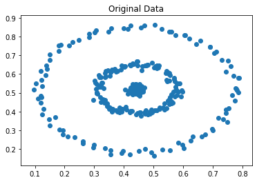
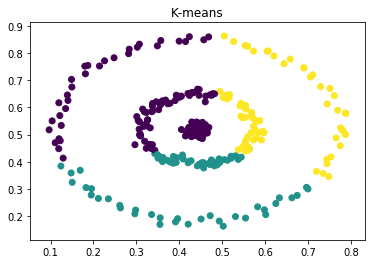
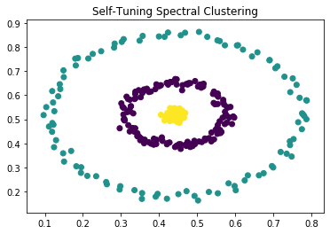
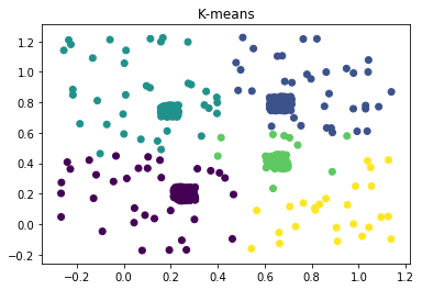
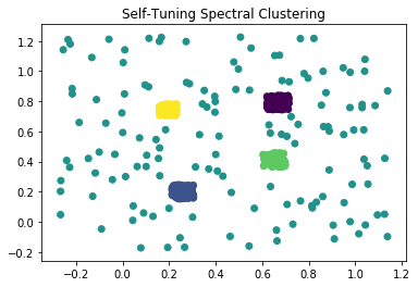
This is a departure from some of the more well-known approaches, such as K-means or learning a mixture model via EM, which are based on the assumption that clusters are concentrated in terms of (often Cartesian) distance. They tend not to do the best when the clusters are of complex or unknown shape, for example -
 |
 |
 |
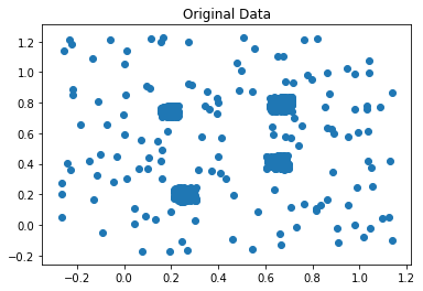
hubs and backgrounds:
 |
 |
 |
Graph Laplacian
The clustering algorithm is made possible by a very handy property of the graph Laplacian.
The Laplacian matrix of a graph \(G\) with \(n\) nodes is defined as
\[L = D - A\]where \(D\) is the degree matrix and \(A\) is the adjacency matrix of graph \(G\). In other words, \(L\) is an \(n \times n\) matrix with elements given by
\[L_{i,j} = \begin{cases} \text{deg}(v_i) & \text{if } i=j \\ -w_{i,j} & \text{if } i \neq j \text{ and there is an edge between i and j }\\ 0 & \text{otherwise } \end{cases}\]If \(G\) is unweighted, we can use \(w_{i,j} = 1\) for each edge.
The property we will be taking advantage of is:
If the graph \(G\) has \(K\) connected components, then \(L\) has \(K\) eigenvectors with an eigenvalue of 0.
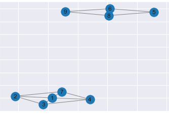
Moreover, the eigenvectors with eigenvalue of 0 are organized in terms of value to indicate the connected components. Here’s an example, with code from Cory Maklin’s blog post:
import networkx as nx
import numpy as np
G = nx.Graph()
G.add_edges_from([[1, 2], [1, 3], [1, 4], [2, 3],
[2, 7], [3, 4], [4, 7], [1, 7],
[6, 5], [5, 8], [6, 8], [9, 8], [9, 6]])
draw_graph(G)
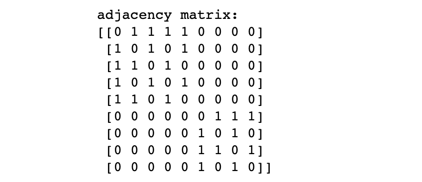
A = nx.adjacency_matrix(G)
print('adjacency matrix:')
print(A.todense())
 |
 |
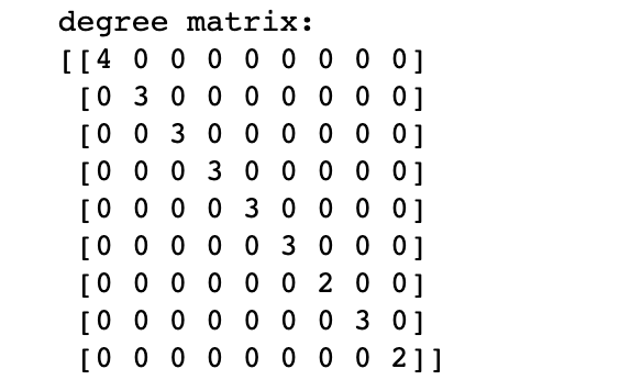
D = np.diag(np.sum(np.array(A.todense()), axis=1))
print('degree matrix:')
print(D)
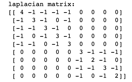
L = D - A
print('laplacian matrix:')
print(L)
 |
 |
Now, if we calculate the eigenvalues and eigenvectors of the Laplacian, we get two 0 eigenvalues as expected. The eigenvectors corresponding to them clearly separate the two clusters. In practice, we use k-means to separate the clusters across the eigenvectors (see section below), as even the clusters are not cleanly separated, the eigenvectors still provide information about interconnectivity.
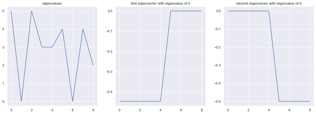 figure 3: concentric circles
TODO: but what does a graph Laplacian and its eigenvectors mean?
Implementing the NJW algorithm
Here we follow Ng, Jordan, and Weiss’s algorithm [2] for (not self-tuning) spectral clustering and implement it step by step. It goes like this:
Given a set of points \(S= \{s_1, \ldots, s_n\}\) in \(\mathbb{R}^l\) and desired number of clusters \(k\):
-
Calculate affinity matrix \(A \in \mathbb{R}^{n \times n}\) defined by
\[A_{ij} = \begin{cases} \exp (- \| s_i - s_j \| ^2 / 2 \sigma^2) & \text{for } i \neq j\\ 0 & \text{for } i=j \end{cases}\]import numpy as np from scipy.spatial.distance import pdist #Calculates pairwise distance def make_A(X, sigma): dim = X.shape[0] A = np.zeros([dim, dim]) dist = iter(pdist(X)) for i in range(dim): for j in range(i+1, dim): d = np.exp(-1*next(dist)**2/(sigma**2)) A[i,j] = d A[j,i] = d return A -
Define \(D\) to be the diagonal matrix whose \((i,i)\) element is the sum of \(A\)’s \(i\)-th row, and construct the Laplacian \(L = D^{-1/2}A D^{-1/2}\).
from scipy import linalg A = make_A(data, 0.3) #Hyper parameter for sigma D = np.sum(A, axis=0) * np.eye(X.shape[0]) D_half = linalg.fractional_matrix_power(D, -0.5) L = np.matmul(np.matmul(D_half, A), D_half) -
Find the \(k\) largest distinct eigenvectors \(x_1, x_2 , \ldots, x_k\) and form the matrix \(X = [x_1x_2\dots x_k]\) by stacking them together as columns.
# numpy returns the eigenvectors as a matrix where the # i-th column corresponds to the i-th eigenvalue. # In the case of all real eigenvalues, they are organized from # small to large. So we are taking the slice of the last k columns. eigval, eigvec = np.linalg.eigh(L) X = eigvec[:, -1*k:] - Re-normalize each row of \(X\) to have unit length. Denote \(Y_{ij} = X_{ij}/(\sum_j X_{ij}^2)^{1/2}\). This step is algorithmically cosmetic and deals with difference of connectivity within a cluster; one may skip this step if that gives better results empirically.
row_sums = Y.sum(axis=1) Y = Y / row_sums[:, np.newaxis] - Cluster each row of \(Y\) into \(k\) clusters by K-means or any other algorithm.
from sklearn.cluster import KMeans clusters = KMeans(n_clusters=k).fit(Y).labels_ - Assign the original point \(s_i\) to the cluster \(j\) where the \(i\)-th row of matrix \(Y\) was assigned to. Implementation-wise, we reuse the
clustersvariable directly.
To finish up, here’s two lines for plotting -
import matplotlib.pyplot as plt

plt.scatter(X[:,0], X[:,1], c = clusters)
plt.title("Spectral Clustering")
Tunning Oneself
Local Scaling
The main drawback of the global \(\sigma\) hyperparameter is that it does not handle the case where data is of various density across the domain, for which a \(\sigma\) may work well with some portion of the data but not the rest. (see figure TODO for example.)
Zelnik-Manor and Perona [1] argues that connectivity/affinity (matrix \(A\)) should be viewed from the points themselves. We can formulate it by selecting a local scaling parameter for each data point \(s_i\). The distance from \(s_i\) to \(s_j\) from the perspective of \(s_i\) is \(d(s_i , s_j )/\sigma_i\) and the converse is \(d(s_i , s_j )/\sigma_j\). The square distance may be generalized as their product, i.e. \(d(s_i , s_j )^2/\sigma_i \sigma_j\). The (local-scaled) affinity between a pair of points therefore becomes:
\[\hat{A}_{ij} = \exp(\frac{-d(s_i,s_j)^2}{\sigma_i\sigma_j})\]Having such construct allows us to adapt the distance -> affinity scaling to data’s local landscape. One way of achieving this goal, as introduced in [1], is to use the local nearest neighbor statistics
\[\sigma_i = d(s_i, s_K)\]Where \(s_K\) is the \(K\)‘th neighbor of \(s_i\). So instead of a graph whose edge weight is absolute distance, we want to construct a weighted nearest neighbor graph. Hyperparameter \(K\) will need to be manually tuned ([1] states that \(K=7\) worked well for all their experiments).
Take data in the following figure for example. The local-scaled affinity will be high between points that are both close neighbors to each other, whereby strongly connecting the red points as in (c) rather than in (b) where a single global \(\sigma\) is used.
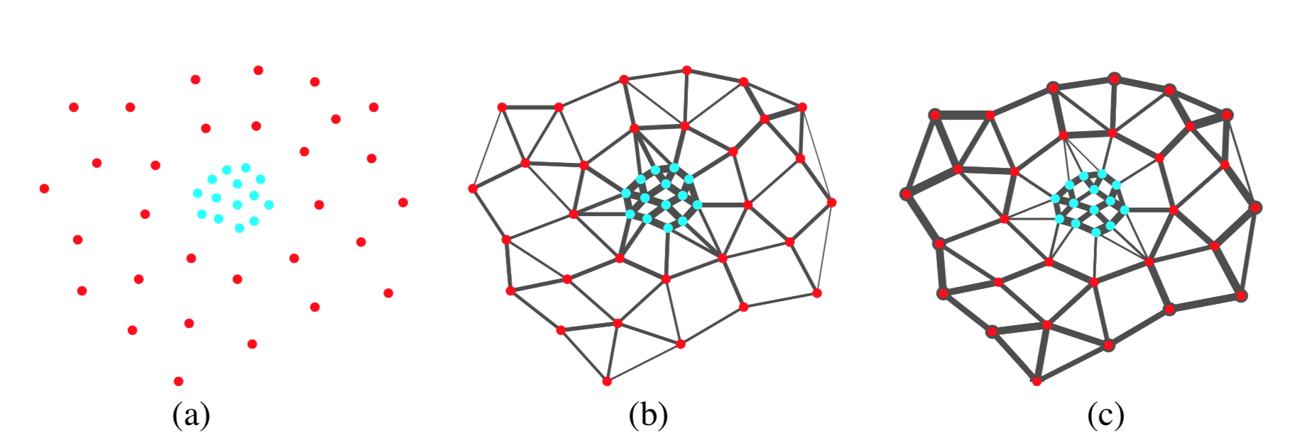 Effect of local scaling, figure 2 from [1]. (a) input data point (b) affinity unscaled, and (c) affinity after local scaling
The implementation of self tuning is straightforward.
from tqdm import tqdm

def A_local(X):
    dim = X.shape[0]
    dist_ = pdist(X)
    pd = np.zeros([dim, dim])
    dist = iter(dist_)
    for i in range(dim):
        for j in range(i+1, dim):
            d = next(dist)
            pd[i,j] = d
            pd[j,i] = d

    #calculate local sigma
    sigmas = np.zeros(dim)
    for i in tqdm(range(len(pd))):
        sigmas[i] = sorted(pd[i])[7]

    A = np.zeros([dim, dim])
    dist = iter(dist_)
    for i in tqdm(range(dim)):
        for j in range(i+1, dim):
            d = np.exp(-1*next(dist)**2/(sigmas[i]*sigmas[j]))
            #print(d)
            A[i,j] = d
            A[j,i] = d
    return A
We can then plug the affinity matrix A into step 2-6 of the NJW algorithm and get results shown in figure 1 and 2.
Estimating number of clusters
So far, all the algorithms we discussed requires the number of cluster as a hyper parameter. In practical cases, however, the optimal number of clusters is often unclear.
Zelnik-Manor and Perona (2014)’s algorithm proposes to use non-maximal suppression after rotating the eigenvector to estimate the number of groups.
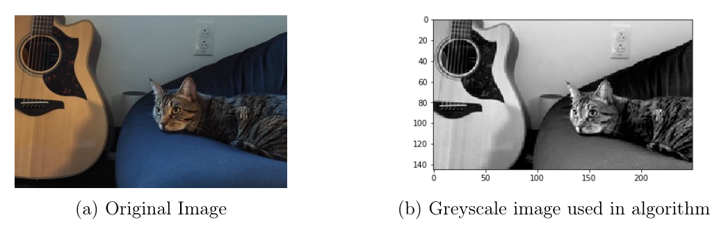
Image Segmentation
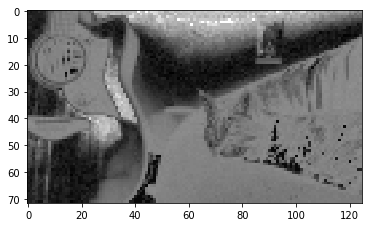
One use case of clustering is on image segmentation. I happen to be cat-sitting for my friend as I’m writing this assignment, so here we go.
 🎸🛋️🐈
🎸🛋️🐈
The way I approached it is to cut the image into smaller patches and cluster them. The code below resizes the image matrix into non-overlapping patches of size \(2×2\), essentially down-sampling the image. open-cv’s python package is used for this processing.
import cv2
from sklearn.feature_extraction import image

im_ = cv2.imread("img_small.jpg", cv2.IMREAD_COLOR)
im = cv2.cvtColor(im_, cv2.COLOR_BGR2GRAY)
plt.imshow(im, cmap = 'gray')

sz = im.itemsize
h,w = im.shape
bh,bw = 2,2 #block height and width
shape = (int(h/bh), int(w/bw), bh, bw)
strides = sz*np.array([w*bh,bw,w,1])
print(shape, strides)

patches = np.lib.stride_tricks.as_strided(im, shape=shape, strides=strides)
Then we apply the algorithm we implemented on the patches. This step is computationally intense and thus time consuming, so I recommend saving the matrices as they are being computed.
a,b,c,d = patches.shape
X = patches.reshape([a*b, c*d])
A = A_local(X)
D_half = linalg.fractional_matrix_power(np.sum(A, axis=0) * np.eye(X.shape[0]), -0.5)
L = np.matmul(np.matmul(D_half, A), D_half)

eigval, eigvec = np.linalg.eigh(L)
we can then plot the eigenvectors.
def eig2pic_(eig):
    arr_blocks = eig.reshape([a, b]) #a, b comes from code block above
    img = np.array([np.hstack(bl) for bl in arr_blocks])
    img = np.vstack(img)
    plt.imshow(img, cmap = 'gray')

eig2pic_(eigvec_cat[:,-1])
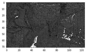 Largest Eigenvector.
Note that the boundaries of the guitar and part of the cat are marked with darker lines, signifying segmentation boundaries. The next few eigenvectors indicates other modes of segmentation:
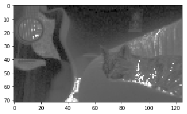 |
 |
 |
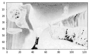
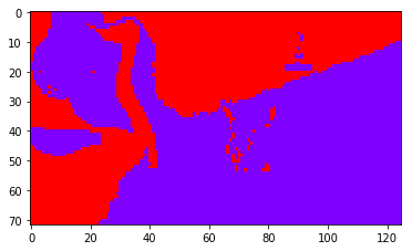
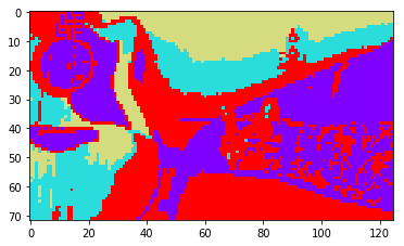
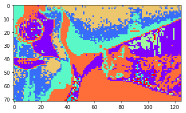
And here are some segmentation results with k-means ran on the first \(k\) eigenvectors, with \(k=2\), \(k=4\), \(k=8\).
 |
 |
 |
Thanks for reading!

References
[1] Lihi Zelnik-Manor, Pietro Perona. “Self-Tuning Spectral Clustering” NeurIPS 2014.
[2] Andrew Ng, Michael Jordan and Yair Weiss. “On spectral clustering: Analysis and an algorithm” NeurIPS 2001.
[3] Carl Doersch, Abhinav Gupta, and Alexei A. Efros. “Unsupervised visual representation learning by context prediction.” ICCV. 2015.