<?xml version="1.0" encoding="utf-8"?><feed xmlns="http://www.w3.org/2005/Atom" ><generator uri="https://jekyllrb.com/" version="3.10.0">Jekyll</generator><link href="https://huiwenn.github.io/feed.xml" rel="self" type="application/atom+xml" /><link href="https://huiwenn.github.io/" rel="alternate" type="text/html" /><updated>2026-05-26T01:39:20+00:00</updated><id>https://huiwenn.github.io/feed.xml</id><title type="html">Sophia Sun</title><subtitle>bleep bloop tech blog.</subtitle><author><name>Sophia Sun</name></author><entry><title type="html">I reviewed for JMLR and all i got is this (not) lousy gif</title><link href="https://huiwenn.github.io/jmlr" rel="alternate" type="text/html" title="I reviewed for JMLR and all i got is this (not) lousy gif" /><published>2025-03-03T00:00:00+00:00</published><updated>2025-03-03T00:00:00+00:00</updated><id>https://huiwenn.github.io/jmlr</id><content type="html" xml:base="https://huiwenn.github.io/jmlr"><![CDATA[<blockquote>
  <p>In support of nice digital artifacts as tokens of appreciation.</p>
</blockquote>

<!--more-->

<p>I submitted a review for a 70 page JMLR manuscript the other day, and they brought me to a page that expressed gratitude and gave me a zip file to download. I openned the zip and found a <code class="language-plaintext highlighter-rouge">README.md</code> file. The readme went:</p>

<div class="language-plaintext highlighter-rouge"><div class="highlight"><pre class="highlight"><code># badges
I review for JMLR badges
</code></pre></div></div>

<p>Here’s the badge in question.</p>

<p><img src="/assets/img/jmlr/I_review_JMLR.gif" alt="" style="width: 40%;" /></p>

<p>cute and/or cringe, seeing it sparked some 2000s internet joy in me.</p>

<p>It also reminded me of <a href="https://danco.substack.com/p/innovation-takes-magic-and-that-magic">Alex Danco’s piece</a> on how science, open sourced software, and startups benifit a lot from gift culture. The reciprocity and goodwill of gift exchange culture (rather than, say, the market of labor and capital) encourages risk-taking and genuine contribution.</p>

<p>Is this badge a gift? It signals that I’m participating in the community around scientific reciprocity, which i proudly displayed in this blog post for vanity. It does not compensate for the 6 hours I spent on it, but is nontheless fulfilling. Maybe one small reason for ML conferences’ disfunctional review system is the lacking of social credits given to reviewers? (I know review experience helps with visa &amp; immigration, but that would not encourage service beyond the needed amount.) Can we start giving out little internet trinkets, unique each year, like ELO badges from games?</p>

<p>I look forward to seeing gifs for reviewers from more ML conferences.</p>]]></content><author><name>Sophia Sun</name></author><category term="misc" /><summary type="html"><![CDATA[In support of nice digital artifacts as tokens of appreciation.]]></summary></entry><entry><title type="html">Learning to Move, Learning to Play, Learning to Animate</title><link href="https://huiwenn.github.io/learning-to-move" rel="alternate" type="text/html" title="Learning to Move, Learning to Play, Learning to Animate" /><published>2024-12-03T00:00:00+00:00</published><updated>2024-12-03T00:00:00+00:00</updated><id>https://huiwenn.github.io/learning-to-move</id><content type="html" xml:base="https://huiwenn.github.io/learning-to-move"><![CDATA[<blockquote>
  <p>An immersive performance featuring multi-modal generative machine learning model @ UCSD’s Qualcomm Institute.</p>
</blockquote>

<!--more-->

<p><img src="/assets/img/yuanque/title.jpg" alt="" /></p>

<p>This is a project funded by UCSD’s Qualcomm institude <a href="https://qi.ucsd.edu/events/learning-to-move-learning-to-play-learning-to-animate/">IDEAS program</a> and is a collaboration with many folks here. See full list of contributors below.</p>

<h3 id="trailer">Trailer</h3>

<iframe width="100%" height="550" src="https://player.vimeo.com/video/966172941" frameborder="0" allow="autoplay; encrypted-media" allowfullscreen=""></iframe>

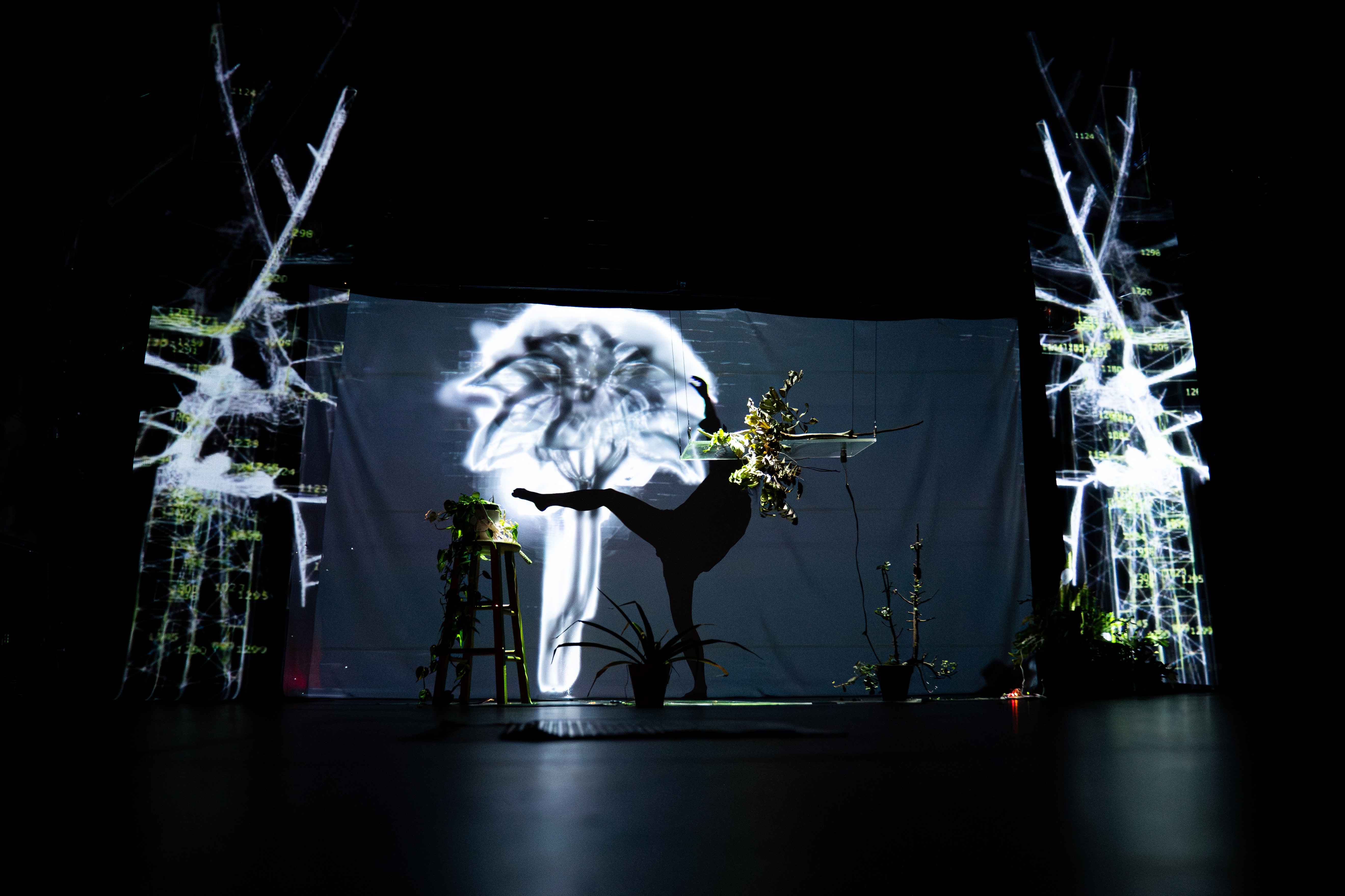
<p>What does it mean to be intelligent? Is it unique to humans, or can it take other forms—beings of wood, stone, metal, and silicon? Recently, we have seen rapid advances in “artificial intelligence,” but its definition has remained elusive. AI systems are often portrayed as some “other,” an alien invention that threatens to overpower us.</p>

<p>At the same time, we are only just becoming aware of the other intelligences surrounding us on this earth, those we’ve failed to recognize or acknowledge for so long. These beings—animals, plants, and natural systems that have been with us all along—are slowly revealing their complexity, agency, and knowledge.</p>

<p>Ecologist and philosopher David Abram coined the phrase “the more-than-human world” to refer to a way of thinking that seeks to override our human tendency to separate ourselves from the natural world. Our work is the artists’ reflection on learning to see technology and nature as part of this more-than-human world. What does it mean to live in a world where we, the technologies we have created, and nature form a collective intelligence? How do we coexist without overpowering or being overpowered by one another?</p>

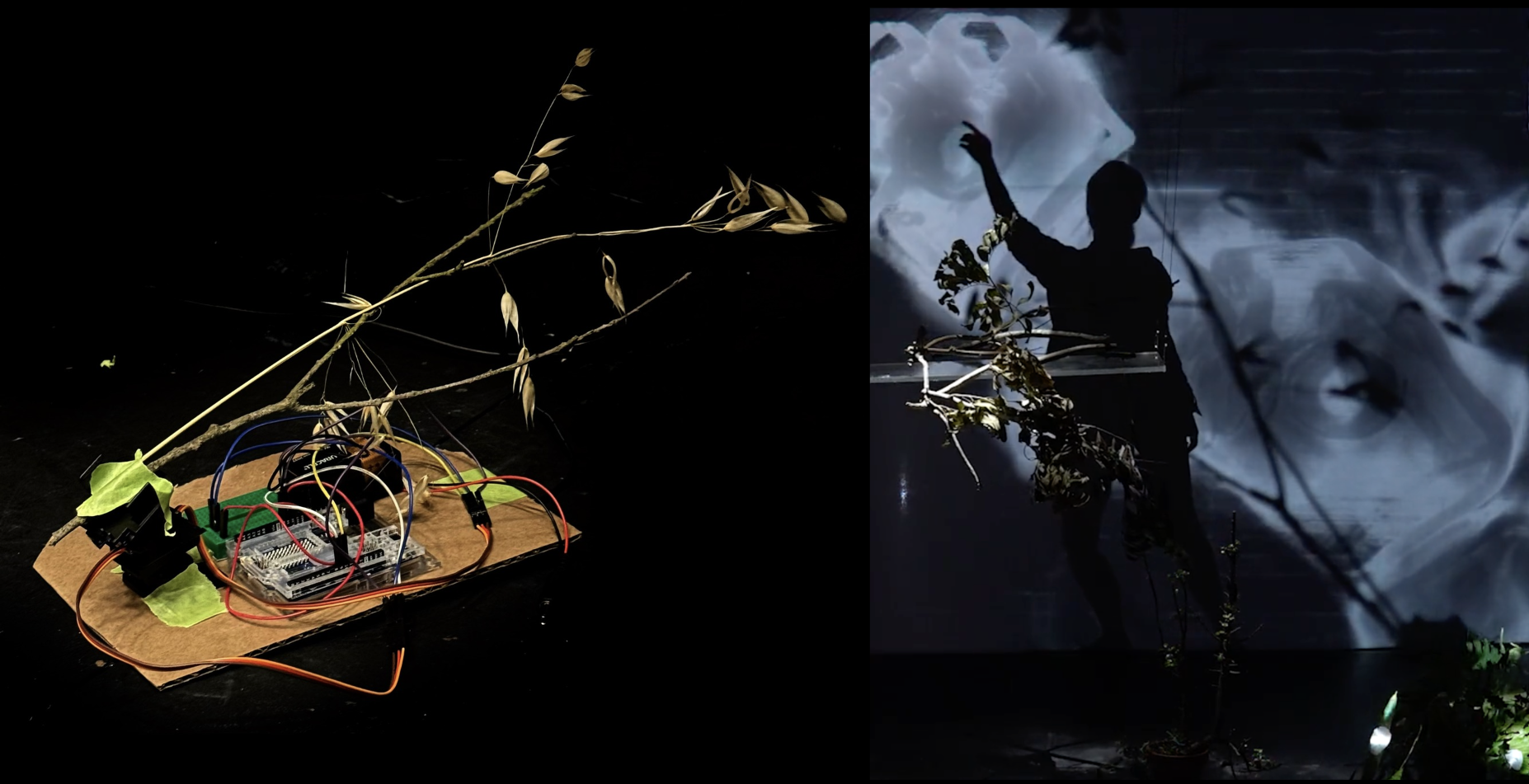
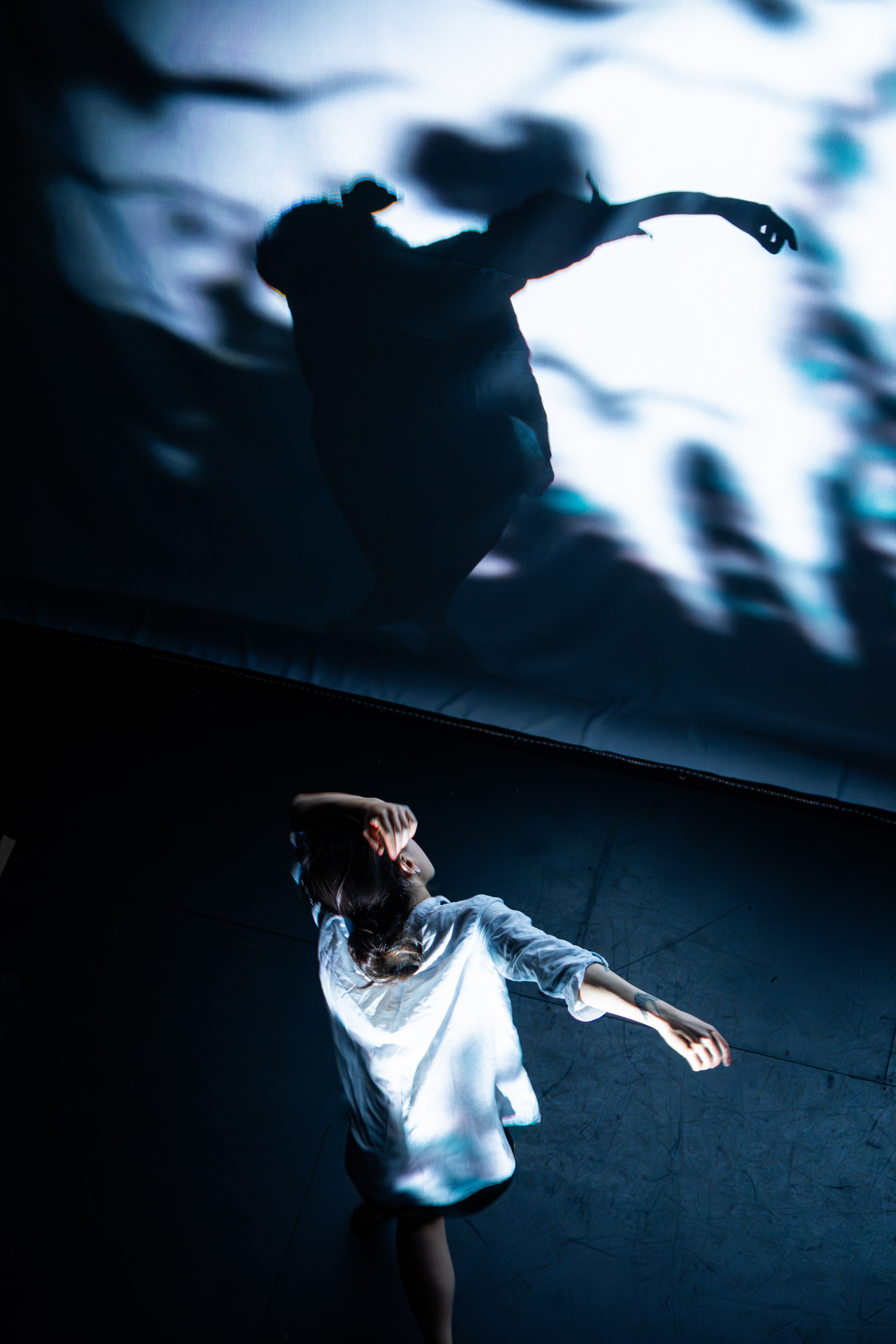
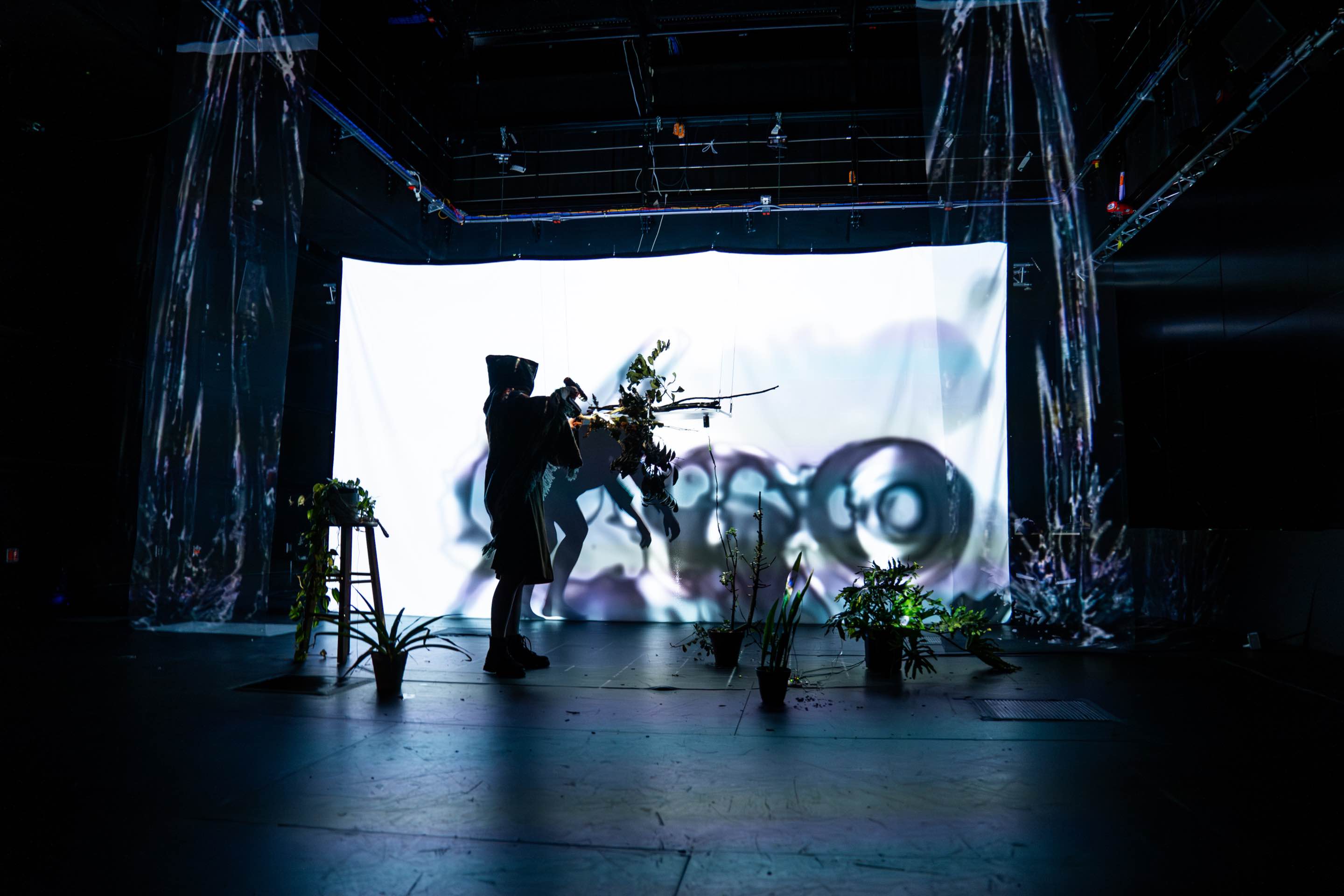
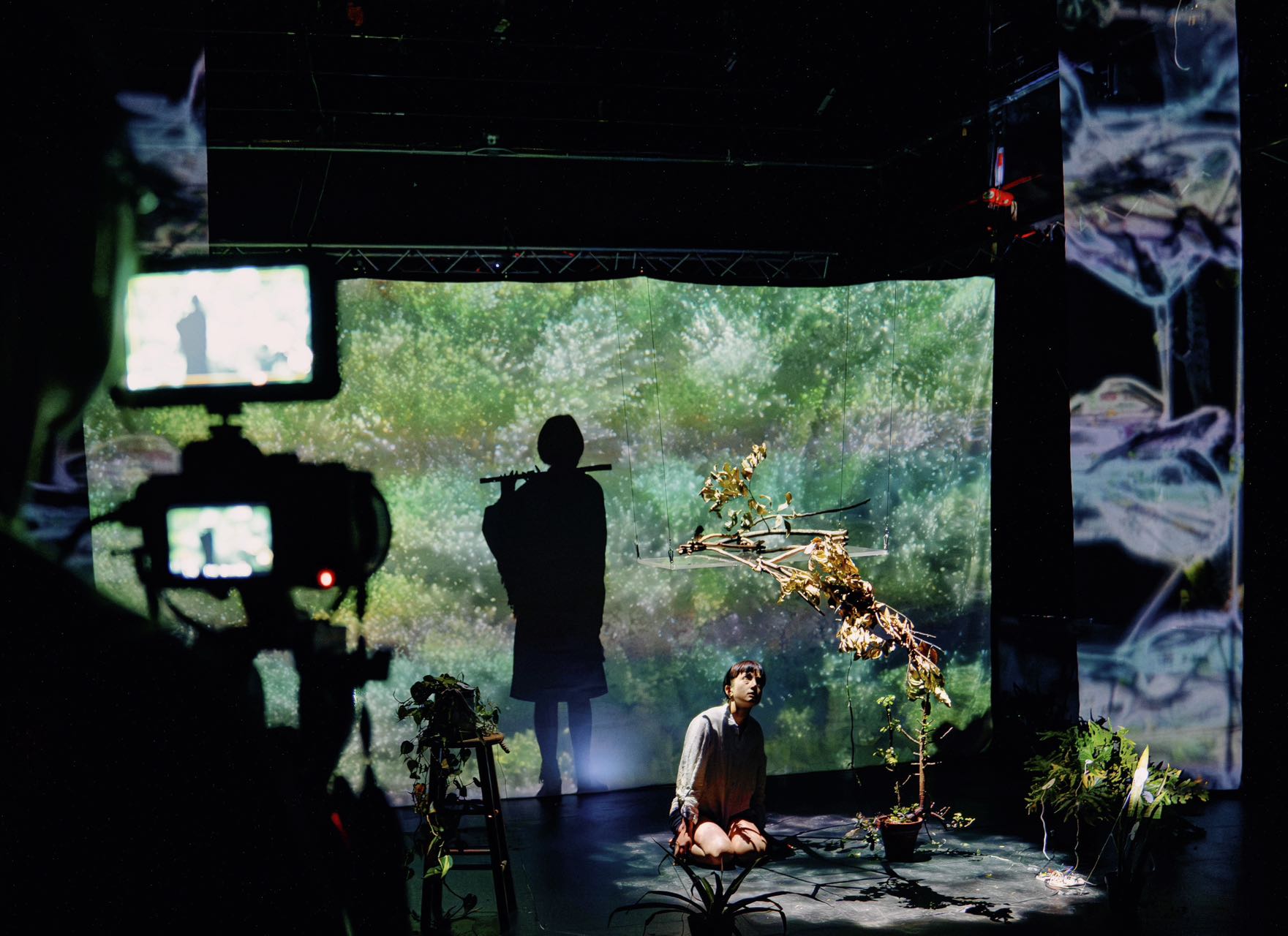
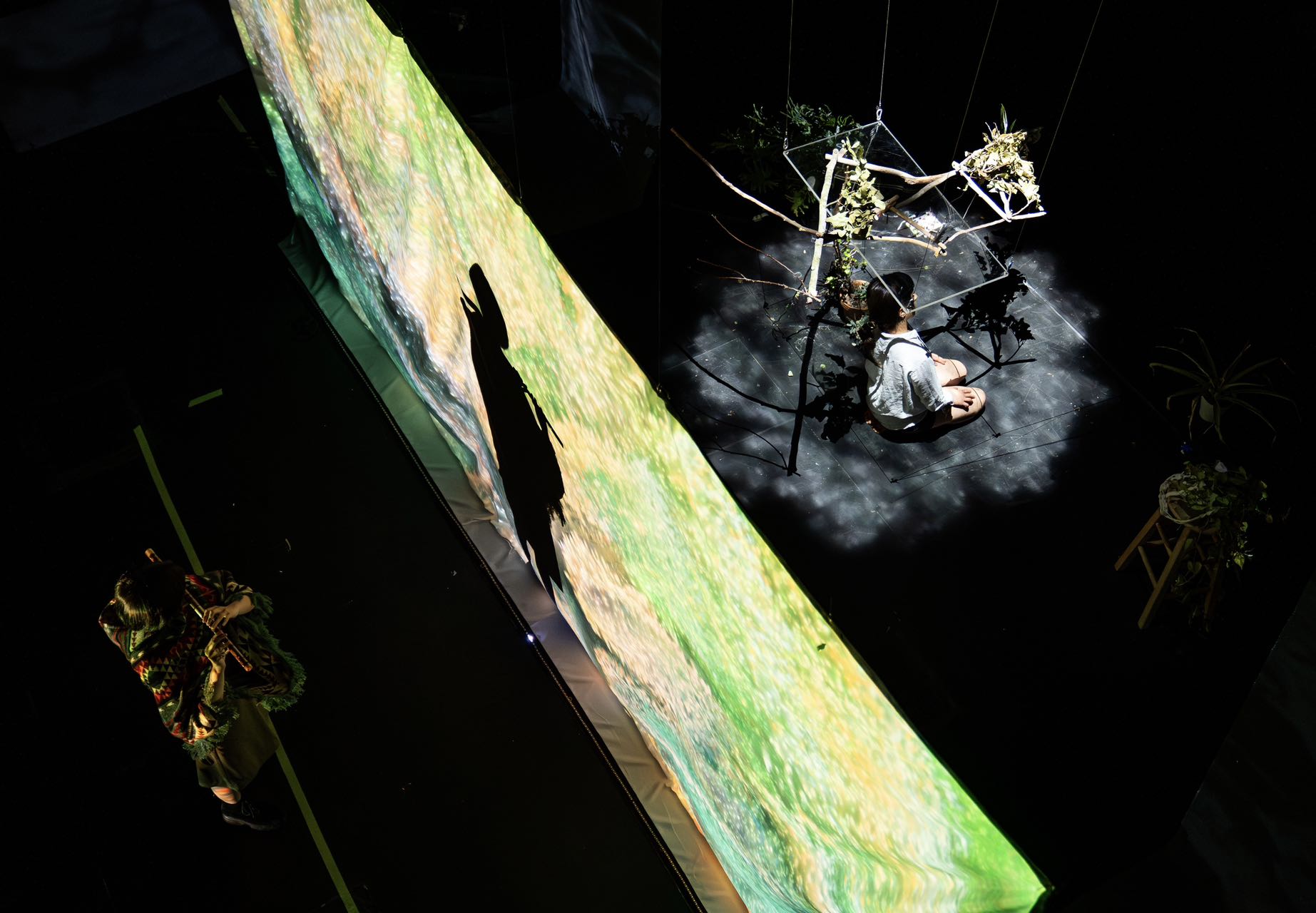
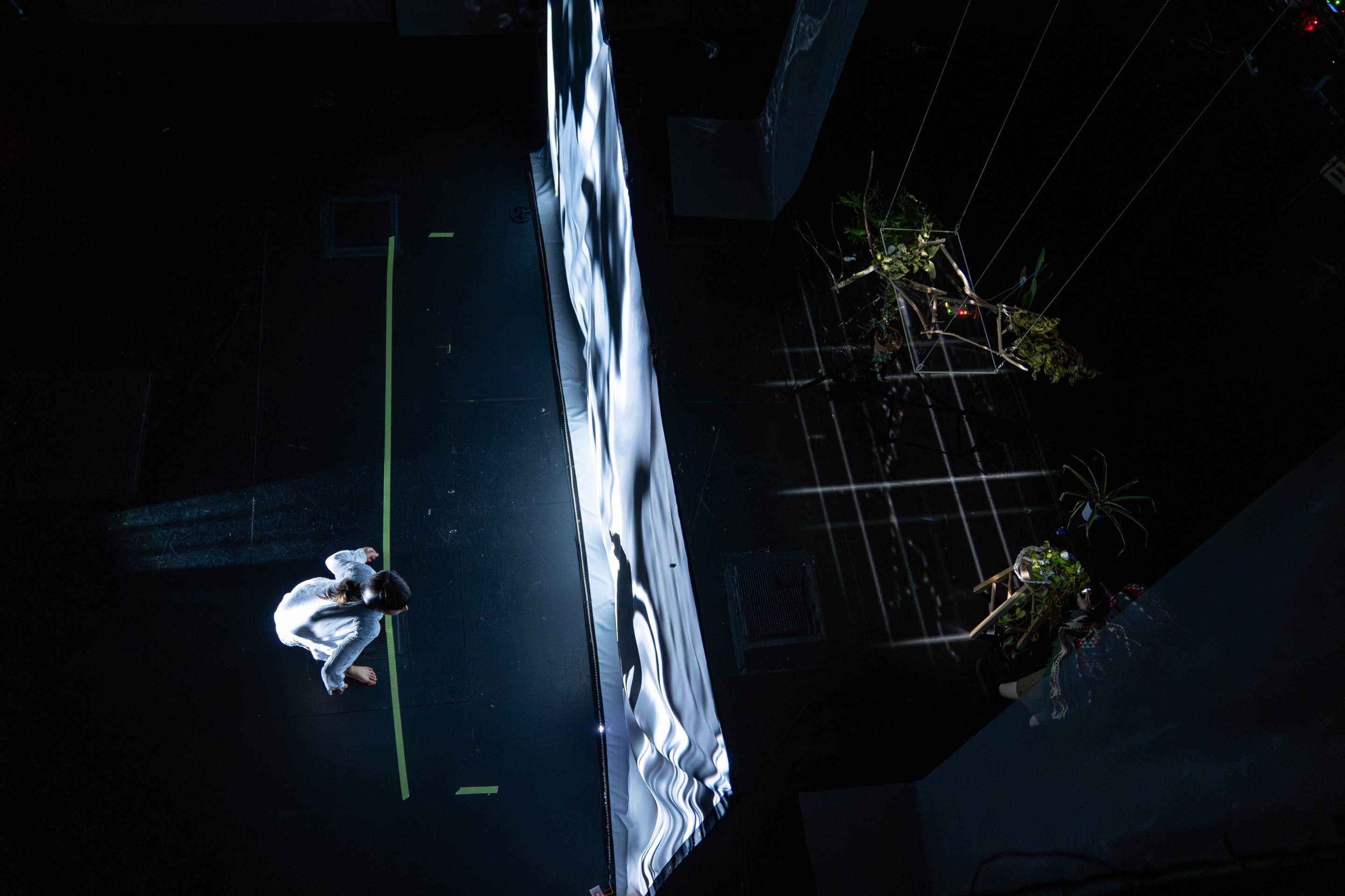
<p>We explore these concepts in our performance through mediums and cutting-edge technologies including self-developed organic material robotics, AI-generated visuals, audio spatialization, real-time bio-feedback data sonification and visualization, and movement. Our performers, machines, and visuals interact in the realm of shadows, whose conceptual framework be traced back to Plato’s allegory of the cave, where shadows on the wall represent the limited and often deceptive nature of human perception. Beginning with mutual imitation and later progressing to playfulness, our performance reflects the complex process of how humans, nature, and machines perceive and learn from one another, reflecting the connected consciousness of our environment, our technologies, and us.</p>

<p> </p>

<h3 id="organic-form-robots">Organic form Robots</h3>

<p><img src="/assets/img/l2m/robot1.png" alt="" />
<em>Large center robot, Jensen’s linkage.</em></p>

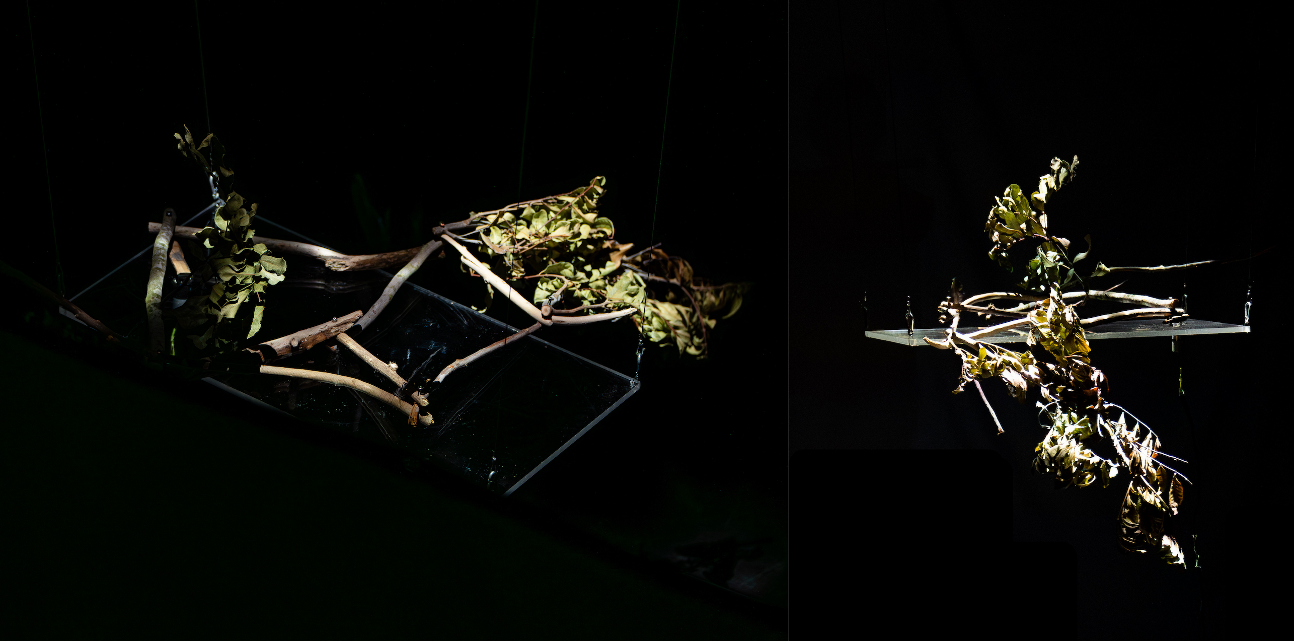
<p><img src="/assets/img/l2m/robot2.png" alt="" />
<em>Arduino IoT controlled organic robot arm, and the shadow it casts.</em></p>
<p> </p>

<h3 id="full-docummentation">Full docummentation:</h3>

<iframe title="vimeo-player" src="https://player.vimeo.com/video/960878340?h=5273aba6fb" width="640" height="360" frameborder="0" allowfullscreen=""></iframe>

<p> </p>

<h4 id="credits">Credits</h4>

<p>(in alphabetical order):</p>

<p>Co-Directors: Mingyong Cheng, Sophia Sun, Han Zhang</p>

<p>Performers: Yuemeng Gu, Erika Roos</p>

<p>Robotic Engineer: Sophia Sun</p>

<p>Visual Artist: Mingyong Cheng</p>

<p>Sound Designer: Han Zhang</p>

<p>Lighting Engineer: Zehao Wang, Han Zhang</p>

<p>Video Editor: Yuemeng Gu</p>

<p>Post Production Coordinator: Mingyong Cheng</p>

<p>Technical &amp; Installation Support: Yifan Guo, Ke Li, Zehao Wang, Zetao Yu</p>

<p>Special thanks to Palka Puri for plant support, the Initiative for Digital Exploration of Arts and Sciences (IDEAS) program at the University of California San Diego and Qualcomm Institute for sponsoring this project, and the AV team from the California Institute for Telecommunications and Information Technology (Calit2) for installation and media support.</p>

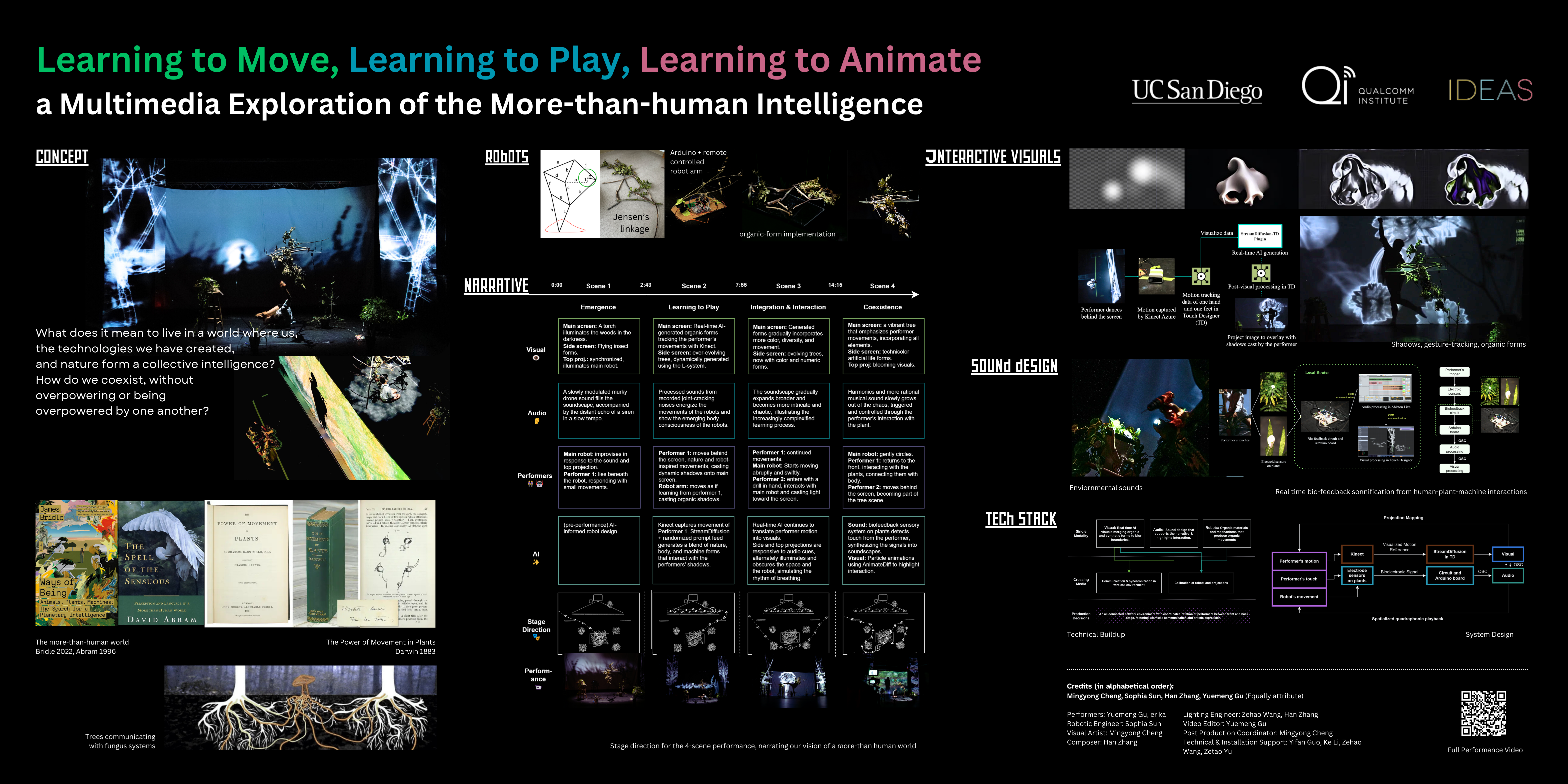
<p><img src="/assets/img/l2m/learning_to_move_poster.png" alt="Poster" />
<em>Poster at Neurips 2024.</em></p>

<p><img src="/assets/img/l2m/1.jpg" alt="stills" />
<img src="/assets/img/l2m/2.jpg" alt="stills" /> 
<img src="/assets/img/l2m/4.jpg" alt="stills" />
<img src="/assets/img/l2m/5.jpg" alt="stills" />
<img src="/assets/img/l2m/6.jpg" alt="stills" />
<img src="/assets/img/l2m/7.jpg" alt="stills" />
<img src="/assets/img/l2m/8.jpg" alt="stills" />
<img src="/assets/img/l2m/9.jpg" alt="stills" /></p>]]></content><author><name>Sophia Sun</name></author><category term="projects" /><category term="machine-learning" /><summary type="html"><![CDATA[An immersive performance featuring multi-modal generative machine learning model @ UCSD’s Qualcomm Institute.]]></summary></entry><entry><title type="html">How to graduate your PhD when you have no hope</title><link href="https://huiwenn.github.io/feynman" rel="alternate" type="text/html" title="How to graduate your PhD when you have no hope" /><published>2024-03-28T00:00:00+00:00</published><updated>2024-03-28T00:00:00+00:00</updated><id>https://huiwenn.github.io/feynman</id><content type="html" xml:base="https://huiwenn.github.io/feynman"><![CDATA[<blockquote>
  <p>a.k.a. Richard Hamming vs. Richard Feynman</p>
</blockquote>

<!--more-->

<p>–</p>

<p>I am going to graduate my phd soon. I’ve been talking to some prospective students recently, and a common question that comes up is: what makes a good phd student? how to be a good researcher?</p>

<p>I’d point them to some <a href="https://huiwenn.github.io/readings">articles</a>, but to be honest I have no idea. What I did spend a lot of time thinking about, and have arrived at a somewhat self-convincing answer, is to a slightly different question - what makes a happy phd student?</p>

<p>The answer is that they are married.</p>

<p>(Obviously this is a joke. We did once survey a 10-phd bbq party, and marriage was the most statistically significant positive correlator. But that’s a story for another time.)</p>

<p>Richard Hamming’s inspiring and influential talk <a href="https://www.cs.virginia.edu/~robins/YouAndYourResearch.html">You and Your Research</a> is what convinced me to do a phd. I wanted to work on important problems and aspired to contribute to the advancement of human knowledge. Oh, to be a scientist! 3 years in I felt like there was no hope; I’ve toiled away all my time and the only way out is to quit.</p>

<p>So I sought advice from my parents. They asked me to think about the least accomplished PhD graduate I know - Can I do as much as they did? What would a minimum effort phd look like? I answered that would result in a pretty bad thesis. And they said, that’s fine, bad is ok, go do what you can. <a href="https://www.poetryfoundation.org/poems/48132/failing-and-flying">Anything worth doing is worth doing badly.</a></p>

<p>And here we are.</p>

<p>This line of reason was put into words a lot more elegantly by Richard Feynman. Allow me to quote his letter in its entirety here - I thought it was the perfect antidote to Hamming-esque anxieties, the Dionysus to our Apollo. Enjoy, and hope you will finish your phd with peacefulness in your heart as well.</p>

<p>–</p>

<p>Dear Koichi,</p>

<p>I was very happy to hear from you, and that you have such a position in the Research Laboratories. Unfortunately your letter made me unhappy for you seem to be truly sad. It seems that the influence of your teacher has been to give you a false idea of what are worthwhile problems. <strong>The worthwhile problems are the ones you can really solve or help solve, the ones you can really contribute something to. A problem is grand in science if it lies before us unsolved and we see some way for us to make some headway into it.</strong> I would advise you to take even simpler, or as you say, humbler, problems until you find some you can really solve easily, no matter how trivial. You will get the pleasure of success, and of helping your fellow man, even if it is only to answer a question in the mind of a colleague less able than you. You must not take away from yourself these pleasures because you have some erroneous idea of what is worthwhile.</p>

<p>You met me at the peak of my career when I seemed to you to be concerned with problems close to the gods. But at the same time I had another Ph.D. Student (Albert Hibbs) was on how it is that the winds build up waves blowing over water in the sea. I accepted him as a student because he came to me with the problem he wanted to solve. With you I made a mistake, I gave you the problem instead of letting you find your own; and left you with a wrong idea of what is interesting or pleasant or important to work on (namely those problems you see you may do something about). I am sorry, excuse me. I hope by this letter to correct it a little.</p>

<p>I have worked on innumerable problems that you would call humble, but which I enjoyed and felt very good about because I sometimes could partially succeed. For example, experiments on the coefficient of friction on highly polished surfaces, to try to learn something about how friction worked (failure). Or, how elastic properties of crystals depends on the forces between the atoms in them, or how to make electroplated metal stick to plastic objects (like radio knobs). Or, how neutrons diffuse out of Uranium. Or, the reflection of electromagnetic waves from films coating glass. The development of shock waves in explosions. The design of a neutron counter. Why some elements capture electrons from the L-orbits, but not the K-orbits. General theory of how to fold paper to make a certain type of child’s toy (called flexagons). The energy levels in the light nuclei. The theory of turbulence (I have spent several years on it without success). Plus all the “grander” problems of quantum theory.</p>

<p>No problem is too small or too trivial if we can really do something about it.</p>

<p>You say you are a nameless man. You are not to your wife and to your child. You will not long remain so to your immediate colleagues if you can answer their simple questions when they come into your office. You are not nameless to me. Do not remain nameless to yourself – it is too sad a way to be. now your place in the world and evaluate yourself fairly, not in terms of your naïve ideals of your own youth, nor in terms of what you erroneously imagine your teacher’s ideals are.</p>

<p>Best of luck and happiness.</p>

<p>Sincerely, Richard P. Feynman.</p>]]></content><author><name>Sophia Sun</name></author><category term="meta-research" /><summary type="html"><![CDATA[a.k.a. Richard Hamming vs. Richard Feynman]]></summary></entry><entry><title type="html">Evaluating Probabilistic Predictions: Proper Scoring Rules</title><link href="https://huiwenn.github.io/predictive-distributions" rel="alternate" type="text/html" title="Evaluating Probabilistic Predictions: Proper Scoring Rules" /><published>2023-10-22T00:00:00+00:00</published><updated>2023-10-22T00:00:00+00:00</updated><id>https://huiwenn.github.io/predictive-distributions</id><content type="html" xml:base="https://huiwenn.github.io/predictive-distributions"><![CDATA[<blockquote>
  <p>Point predictions are often insufficient for machine learning tasks that involves uncertainty. As a solution, probabilistic models are becoming more widely used. This post talks about proper scoring rules, a framework to think about and evaluate probabilistic predictions.</p>
</blockquote>

<!--more-->

<ul class="table-of-content" id="markdown-toc">
  <li><a href="#probabilistic-predictions--predictive-distributions" id="markdown-toc-probabilistic-predictions--predictive-distributions">Probabilistic Predictions / Predictive Distributions</a>    <ul>
      <li><a href="#calibration-and-accuracy" id="markdown-toc-calibration-and-accuracy">Calibration and Accuracy</a></li>
    </ul>
  </li>
  <li><a href="#proper-scoring-rules-psr" id="markdown-toc-proper-scoring-rules-psr">Proper Scoring Rules (PSR)</a>    <ul>
      <li><a href="#definition" id="markdown-toc-definition">Definition</a></li>
      <li><a href="#common-scoring-rules" id="markdown-toc-common-scoring-rules">Common Scoring Rules</a>        <ul>
          <li><a href="#negative-log-likelihood-nll" id="markdown-toc-negative-log-likelihood-nll">Negative Log Likelihood (NLL)</a></li>
          <li><a href="#brierquadratic-score" id="markdown-toc-brierquadratic-score">Brier/Quadratic Score</a></li>
          <li><a href="#continuous-ranked-probability-score-crps" id="markdown-toc-continuous-ranked-probability-score-crps">Continuous Ranked Probability Score (CRPS)</a></li>
          <li><a href="#energy-score" id="markdown-toc-energy-score">Energy Score</a></li>
          <li><a href="#interval-specific-mean-interval-score" id="markdown-toc-interval-specific-mean-interval-score">Interval specific: Mean Interval Score</a></li>
          <li><a href="#interval-specific-winkler-score" id="markdown-toc-interval-specific-winkler-score">Interval specific: Winkler Score</a></li>
          <li><a href="#tangent-is-kl-divergence-a-proper-scoring-rule" id="markdown-toc-tangent-is-kl-divergence-a-proper-scoring-rule">tangent: Is KL divergence a proper scoring rule?</a></li>
        </ul>
      </li>
    </ul>
  </li>
  <li><a href="#discussion" id="markdown-toc-discussion">Discussion</a></li>
</ul>

<h2 id="probabilistic-predictions--predictive-distributions">Probabilistic Predictions / Predictive Distributions</h2>

<p>Predictive distributions are when a model produces a probability distribution (as opposed to a point prediction) given data and parameters. They have many benefits - many real world problems have inherent uncertainty, and we can capture thing we care about, like risk or reward, through a probabilistic representation. With predictive distributions, we can have better uncertainty quantification, and make better decisions given these uncertainties.</p>

<p>To put in perspective, for input \(X\), instead of outputting a point prediction \(y\), the model outputs a distribution over the space of outputs \(p(y\vert X)\).</p>

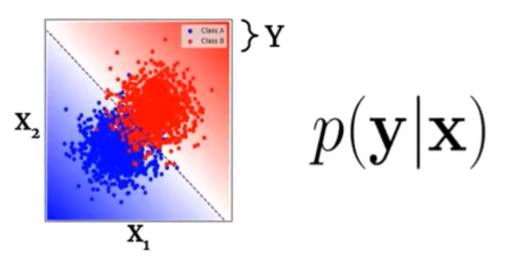
<p>For example, for a classification task, we can output confidence along with a label:</p>

<p><img src="/assets/img/properscoring/classification.png" alt="" style="width: 60%;" /></p>

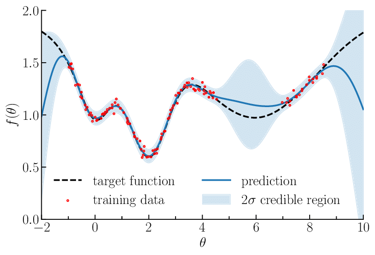
<p>For regression, one can output a gaussian distribution over \(y\) (mean and variance), like in the case of Gaussian Process regression:</p>

<p><img src="/assets/img/properscoring/gp.png" alt="" style="width: 60%;" /></p>

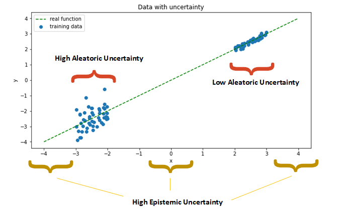
<p>Uncertainties can be from different sources. The most mainstream distinction is aleatoric (there exists variations in the data, as in our classification example) vs epistemic (we don’t have enough data to know the label for sure, as in our regression example).</p>

<p><img src="/assets/img/properscoring/uq.png" alt="Illustration from talk by Balaji Lakshminarayanan, Dustin Tran, and Jasper Snoek from Google Brain" style="width: 90%;" /></p>

<h3 id="calibration-and-accuracy">Calibration and Accuracy</h3>

<p>In general, we want two thing from our probabilistic forecasts: calibration, and accuracy. Calibration refers to that the probabilities predicted actually corresponds to the true probabilities. For example,  among the days that we predict 30% precipitation rate, 30% of them actually rained.</p>

<p>In the machine learning community, many studies have shown that as neural networks get deeper, they become less calibrated. So there have been efforts to calibrating neural networks using techniques like <a href="https://papers.nips.cc/paper_files/paper/2017/hash/9ef2ed4b7fd2c810847ffa5fa85bce38-Abstract.html">ensembles</a> and <a href="http://proceedings.mlr.press/v70/guo17a.html">temporal scaling</a>, among others. This is still an active area of study.</p>

<p>An important note is that calibration is not the same thing as accuracy. A model can be perfectly calibrated but completely useless - for example, for a binary classification task with a balanced test set, a model that predicts class A always with \(50\%\) probability.</p>

<p>Evaluating probabilistic forecasts, then, requires evaluating both accuracy and calibration. This is where proper scoring rules come in.</p>

<h2 id="proper-scoring-rules-psr">Proper Scoring Rules (PSR)</h2>

<h3 id="definition">Definition</h3>

<p>Scoring rules are functions that score how well a predictive distribution captures data. Let’s say we have data domain \(x \sim \mathbf{X}\), and \(P\) is a distribution over \(\mathbf{X}\). Then the score</p>

\[S: P \times x \rightarrow \mathbb{R}\]

<p>It assess the quality of probabilistic forecasts, by assigning a numerical score based on the predictive distribution and on the event or value that materializes. A scoring rule is proper if the forecaster maximizes the expected score for an observation drawn from the distribution \(F\) if he or she issues the probabilistic forecast \(F\), rather than \(G = F\). It is strictly proper if the maximum is unique.</p>

<h3 id="common-scoring-rules">Common Scoring Rules</h3>

<h4 id="negative-log-likelihood-nll">Negative Log Likelihood (NLL)</h4>

<p>You probably know what NLL is. In addition to being a proper scoring rule, it also have optimal discrimination power.</p>

\[NLL = -\sum_{i=1}^{n} \left[ y_i \log(p(y_i)) + (1 - y_i) \log(1 - p(y_i)) \right]\]

<h4 id="brierquadratic-score">Brier/Quadratic Score</h4>

<p>Brier score is a PSR for classification tasks. It is sometimes preferred over NLL because it is bounded within \([0,1]\) and hence more stable.</p>

<p>In the binary setting, we can calculate it as:</p>

\[BS = \frac{1}{n} \sum_{i=1}^{n} (p_i - o_i)^2\]

<ul>
  <li>\(n\) is the total number of observations or data points.
​</li>
  <li>
    <p>\(p_i\) represents the predicted probability of the positive class for the i-th observation.</p>
  </li>
  <li>\(o_i\) is an indicator variable that equals 1 if the event occurred and 0 if it did not for the 
i-th observation.</li>
</ul>

<h4 id="continuous-ranked-probability-score-crps">Continuous Ranked Probability Score (CRPS)</h4>

<p>Continuous Ranked Probability Score (CRPS) is another metric widely used in fields like meteorology, hydrology, and climate science. In plain words, the CRPS measures the discrepancy between the predicted cumulative distribution function (CDF) of a forecast and a step function representing the true outcome. It essentially quantifies the spread of the forecast distribution around the observed value.</p>

<p>The Continuous Ranked Probability Score is defined as:</p>

\[CRPS(F, y) = \int_{-\infty}^{\infty} [F(x) - \mathbb{1}(x \geq y)]^2 \, dx\]

<ul>
  <li>\(CRPS(F, y)\): The Continuous Ranked Probability Score for the forecast \(F\) and the observed outcome \(y\).</li>
  <li>\(F(x)\): The cumulative distribution function (CDF) of the forecast, evaluated at \(x\).</li>
  <li>\(\mathbb{1}(x \geq y)\): The indicator function which equals 1 if \(x \geq y\) and 0 otherwise.</li>
  <li>\(dx\): Infinitesimal change in \(x\), indicating integration over the entire real number line.</li>
</ul>

<h4 id="energy-score">Energy Score</h4>
<p>Energy Score (ES) is a proper scoring rule to measure calibration and sharpness of the predicted distributions. Defined as</p>

\[\text{ES}(P, \textbf{x}) = E_{ \textbf{X} \sim P} \| \textbf{X} - \textbf{x} \| - \frac{1}{2} E_{ \textbf{X, X'} \sim P} \| \textbf{X} - \textbf{X'} \|\]

<p><a href="https://arxiv.org/pdf/2010.03759.pdf">This paper</a> shows that the energy score outperforms the softmax confidence score on common OOD evaluation benchmarks.</p>

<p>The energy score is parameter-free measure, which makes it easy to implement, especially for distributions whose analytic expressions are unavailable or difficult. Another result of this property is that it is not directly differentiable w.r.t. parameters.</p>

<h4 id="interval-specific-mean-interval-score">Interval specific: Mean Interval Score</h4>

<p>A common way of using probability forecasts for decision making is translating it to confidence intervals. We will go through two of the</p>

<p>The Mean Interval Score is a metric used to evaluate the accuracy and calibration of probabilistic forecasts. It measures the average width of prediction intervals relative to the observed outcomes.</p>

<p>Keep in mind that this is a specialized metric for evaluating prediction intervals, and it may not be as commonly used as metrics like Brier score or log-likelihood in all contexts.</p>

<p>In a prediction interval, a model not only predicts a point estimate but also provides a range of values within which the actual outcome is expected to fall with a certain confidence level.</p>

<p>The Mean Interval Score is defined as follows:</p>

\[MIS = \frac{1}{n} \sum_{i=1}^{n} (U_i - L_i) + \frac{2}{\alpha} \sum_{i=1}^{n} (L_i - y_i)1_{y_i &lt; L_i} + \frac{2}{\alpha} \sum_{i=1}^{n} (y_i - U_i)1_{y_i &gt; U_i}\]

<p>Where:</p>

<ul>
  <li>\(n\) is the total number of observations or data points.</li>
  <li>\(U_i\) is the upper bound of the prediction interval for the i-th observation.</li>
  <li>\(L_i\) is the lower bound of the prediction interval for the i -th observation.</li>
  <li>\(y_i\) is the actual observed value for the \(i\)-th observation.</li>
  <li>\(\alpha\) is the confidence level of the prediction interval (e.g., 0.95 for a 95% confidence interval).</li>
  <li>\(I(\cdot)\) is the indicator function, which equals 1 if the condition inside the parentheses is true, and 0 otherwise.</li>
</ul>

<p>The Mean Interval Score penalizes prediction intervals that are too wide or too narrow compared to the actual outcomes. It also accounts for cases where the actual outcome falls outside the predicted interval.</p>

<h4 id="interval-specific-winkler-score">Interval specific: Winkler Score</h4>

<p>The Winkler score is another fun one for confidence intervals / regions, and can be easily extended to forecasts in higher dimensions. It is essentially a a metric measuring the overlap between two sets.</p>

\[WS = \frac{2 \times |A \cap B|}{|A| + |B|}\]

<p>where \(A\) and \(B\) are binary sets and | \(\cdot\) | denotes the cardinalities of the sets.</p>

<p>The Winkler Score ranges from 0 to 1, with 1 indicating complete overlap and 0 indicating no overlap between the sets.</p>

<h4 id="tangent-is-kl-divergence-a-proper-scoring-rule">tangent: Is KL divergence a proper scoring rule?</h4>

<p>No. The main difference between KL divergence (and other entropy metrics) as opposed to PSRs is that it measures difference between two distributions, where as PSRs calculates a score with the predictive distribution and <em>observations</em>. Often we do not have the ground truth distribution, so we would have to approximate the KL divergence.</p>

<p>KL is also not <em>strictly</em> proper: While KL divergence is proper in the sense that it is minimized when the predicted distribution matches the true distribution, it is not strictly proper because it doesn’t have a unique maximum. In other words, multiple predicted distributions can yield the same KL divergence value.</p>

<p>This is not to say that we should not use KL divergence as a measure of accuracy. It is very helpful for optimization and model selection because of its sensitivity to small differences, and can be used along with other PSRs.</p>

<h2 id="discussion">Discussion</h2>

<p>I hope I’ve made the case for using proper scoring rules as evaluators of probabilistic predictions, and provided a  grimoire of useful scores.</p>

<p>It is worth noting that, while being <em>proper</em> is  helpful for model comparison, it is just one of the desirable property for a metric. <a href="https://proceedings.mlr.press/v202/marcotte23a/marcotte23a.pdf">This paper</a> from ICML 2023 raised the important point that we also need to pay attention to metric’s discriminative performance in the settings of the task. They showed that in a multivariate time series forecasting context, the energy score and CRPS fail to capture correlation structures between the variables, and are not sensitive to discrepancies in higher moments. Some scoring rules also appears complementary in their discriminative emphases, so it is worth having an ensemble of metrics for reliably measuring the correctness of forecasts.</p>

<p>Happy hacking!</p>

<hr />

<p><em>Extended Readings</em></p>

<ul>
  <li>
    <p><a href="https://sites.stat.washington.edu/raftery/Research/PDF/Gneiting2007jasa.pdf">Strictly proper scoring rules, prediction, and estimation.</a>. Gneiting, Tilmann, and Adrian E. Raftery. The OG proper scoring rules paper.</p>
  </li>
  <li>
    <p><a href="https://arxiv.org/pdf/2107.00363.pdf">Valid prediction intervals for regression problems</a>. Nicolas Dewolf, Bernard De Baets, Willem Waegeman. A survey of probablistic forecasting models including Bayesian methods (GP, BNN), ensemble methods, direct estimation methods (quantile regression), and conformal prediction methods. They introduce the methods clearly and compare the advantages and disadvantages of each.</p>
  </li>
</ul>

<hr />

<p><em>References</em></p>

<p>Michel Kana, “Uncertainty in Deep Learning. How To Measure?” <a href="https://towardsdatascience.com/my-deep-learning-model-says-sorry-i-dont-know-the-answer-that-s-absolutely-ok-50ffa562cb0b">blogpost</a>, 2020</p>

<p>Balaji Lakshminarayanan, Dustin Tran,  and Jasper Snoek, “Uncertainty and Out-of-Distribution Robustness in Deep Learning” Talk at NERSC <a href="https://www.youtube.com/watch?v=ssD7jNDIL2c&amp;ab_channel=NERSC">youtube</a>, 2020</p>

<p>Gneiting, Tilmann, and Adrian E. Raftery. “Strictly proper scoring rules, prediction, and estimation.” <a href="https://sites.stat.washington.edu/raftery/Research/PDF/Gneiting2007jasa.pdf">pdf</a> <em>Journal of the American statistical Association</em> 102.477 (2007): 359-378.</p>

<p>Victor Richmond Jose, Robert Nau, &amp; Robert Winkler. “Scoring Rules, Generalized Entropy, and Utility Maximization” <a href="https://people.duke.edu/~rnau/Nau_Scoring_Rules_Paris_seminar.pdf">slides</a>, Presentation for GRID/ENSAM Seminar, 2007</p>

<p>Marcotte, Étienne, Valentina Zantedeschi, Alexandre Drouin, and Nicolas Chapados. “Regions of Reliability in the Evaluation of Multivariate Probabilistic Forecasts.” <a href="https://proceedings.mlr.press/v202/marcotte23a/marcotte23a.pdf">pdf</a> ICML 2023</p>]]></content><author><name>Sophia Sun</name></author><category term="machine-learning" /><summary type="html"><![CDATA[Point predictions are often insufficient for machine learning tasks that involves uncertainty. As a solution, probabilistic models are becoming more widely used. This post talks about proper scoring rules, a framework to think about and evaluate probabilistic predictions.]]></summary></entry><entry><title type="html">Synthetic Erudition Assist Lattice</title><link href="https://huiwenn.github.io/seals" rel="alternate" type="text/html" title="Synthetic Erudition Assist Lattice" /><published>2021-05-27T00:00:00+00:00</published><updated>2021-05-27T00:00:00+00:00</updated><id>https://huiwenn.github.io/seals</id><content type="html" xml:base="https://huiwenn.github.io/seals"><![CDATA[<!--more-->

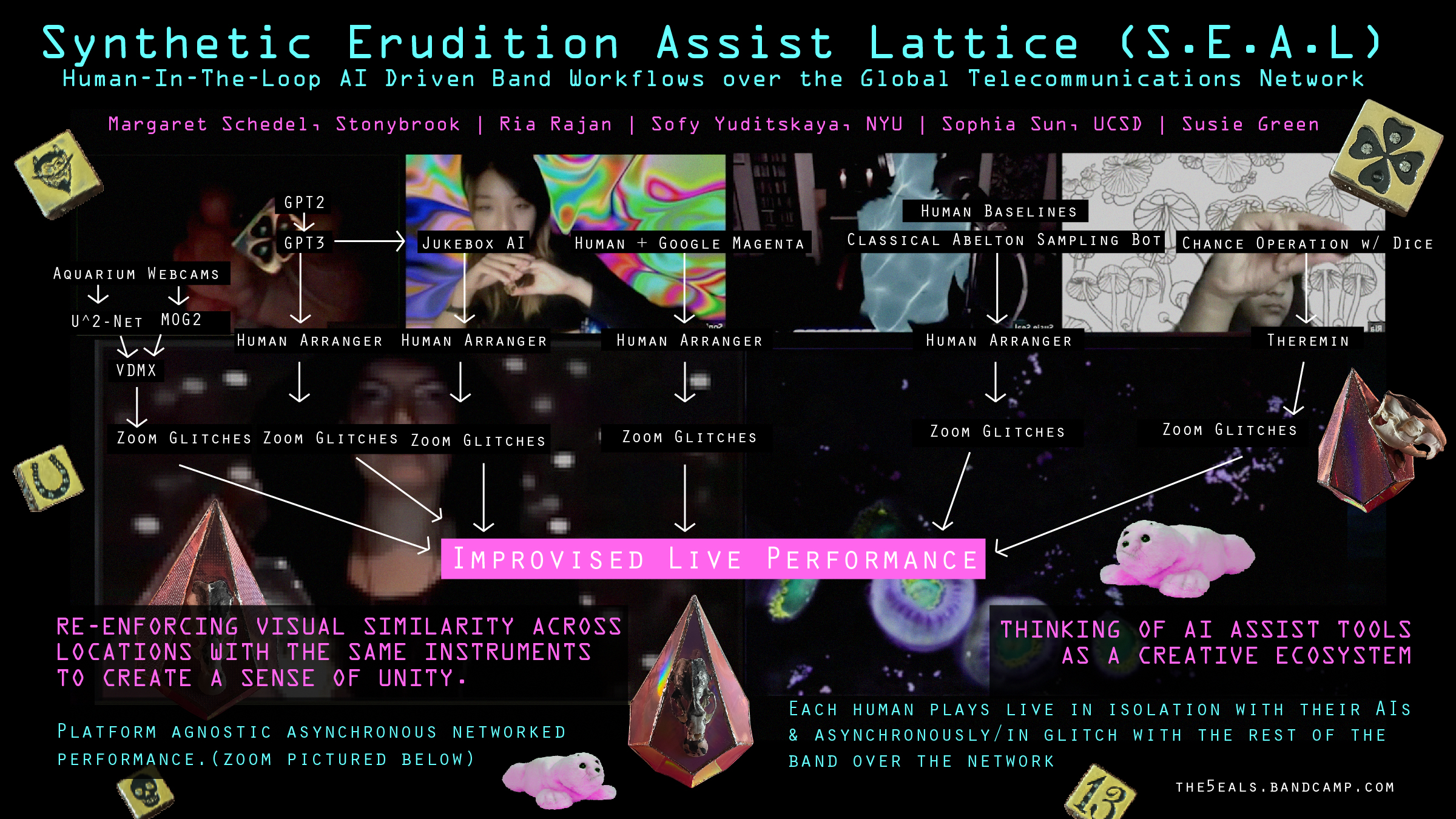
<p><img src="/assets/img/seals/seals.jpg" alt="" /></p>

<p>Update: We presented ur music video for <em>Lockdown</em> at the <a href="https://neuripscreativityworkshop.github.io/2022/">Machine Learning for Creativity and Design Workshop</a> at NeurIPS 2022.</p>

<p><em>our poster for NIME 2021</em>
 </p>

<p>You can read the paper <a href="https://nime.pubpub.org/pub/5oupvoun/draft?access=jhkokrol">here</a> and listen to our music <a href="https://the5eals.bandcamp.com/album/the-seals-holiday-special">here</a>.</p>

<p>This paper documents the music-making of the band <em>Seals</em>, for which I play bass and do machine learning. The Seals is a pet project with Margaret Schedel, Susie Green, Ria Rajan, and Sofy Yuditskaya; we introduce ourselves, (cheekly), as <em>a political, feminist, noise, and AI-inspired electronic sorta-surf rock band</em>. The S.E.A.L. (Synthetic Erudition Assist Lattice) is the collection of algorithms that assist us in creating content with which to mold and shape our music and visuals. Glad to see our acronym powers from academia came into use.</p>

<p>Our first collection of songs are about how our living experiences are mediated by technology, pandemic lockdowns, the female body, and the occult.  I hope we can bring a performance to you one day.</p>

<p> </p>

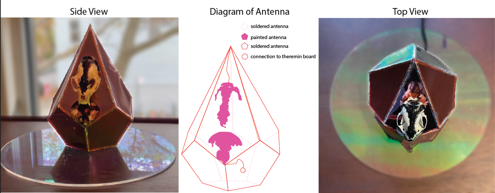
<p><img src="/assets/img/seals/theremin.png" alt="" style="width: 80%;" class="center" />
<em>Sofy made custom theremins for all of us.</em>
 </p>]]></content><author><name>Sophia Sun</name></author><category term="projects" /><summary type="html"><![CDATA[]]></summary></entry><entry><title type="html">Found Materials Drawing Machine</title><link href="https://huiwenn.github.io/drawingmachine" rel="alternate" type="text/html" title="Found Materials Drawing Machine" /><published>2020-07-01T01:09:00+00:00</published><updated>2020-07-01T01:09:00+00:00</updated><id>https://huiwenn.github.io/drawingmachine</id><content type="html" xml:base="https://huiwenn.github.io/drawingmachine"><![CDATA[<!--more-->

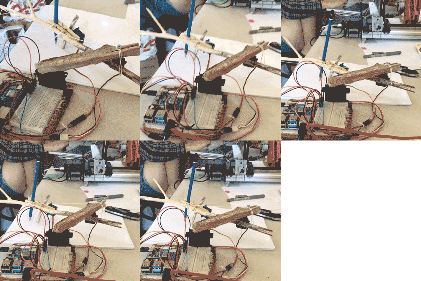
<p style="width: 60%;" class="center"><img src="/assets/img/drawingmachine/vid.gif" alt="robot" /></p>
<p> </p>

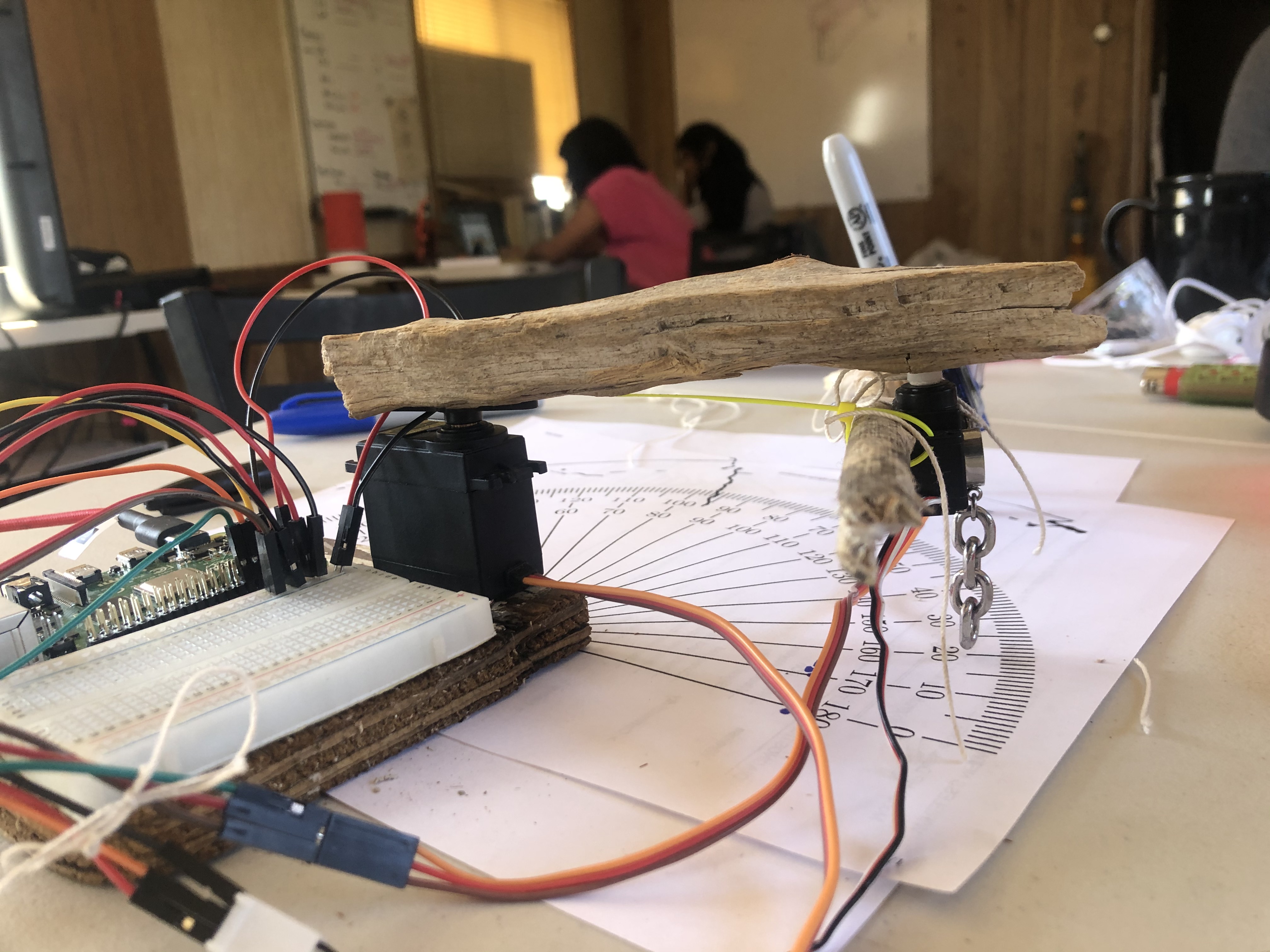
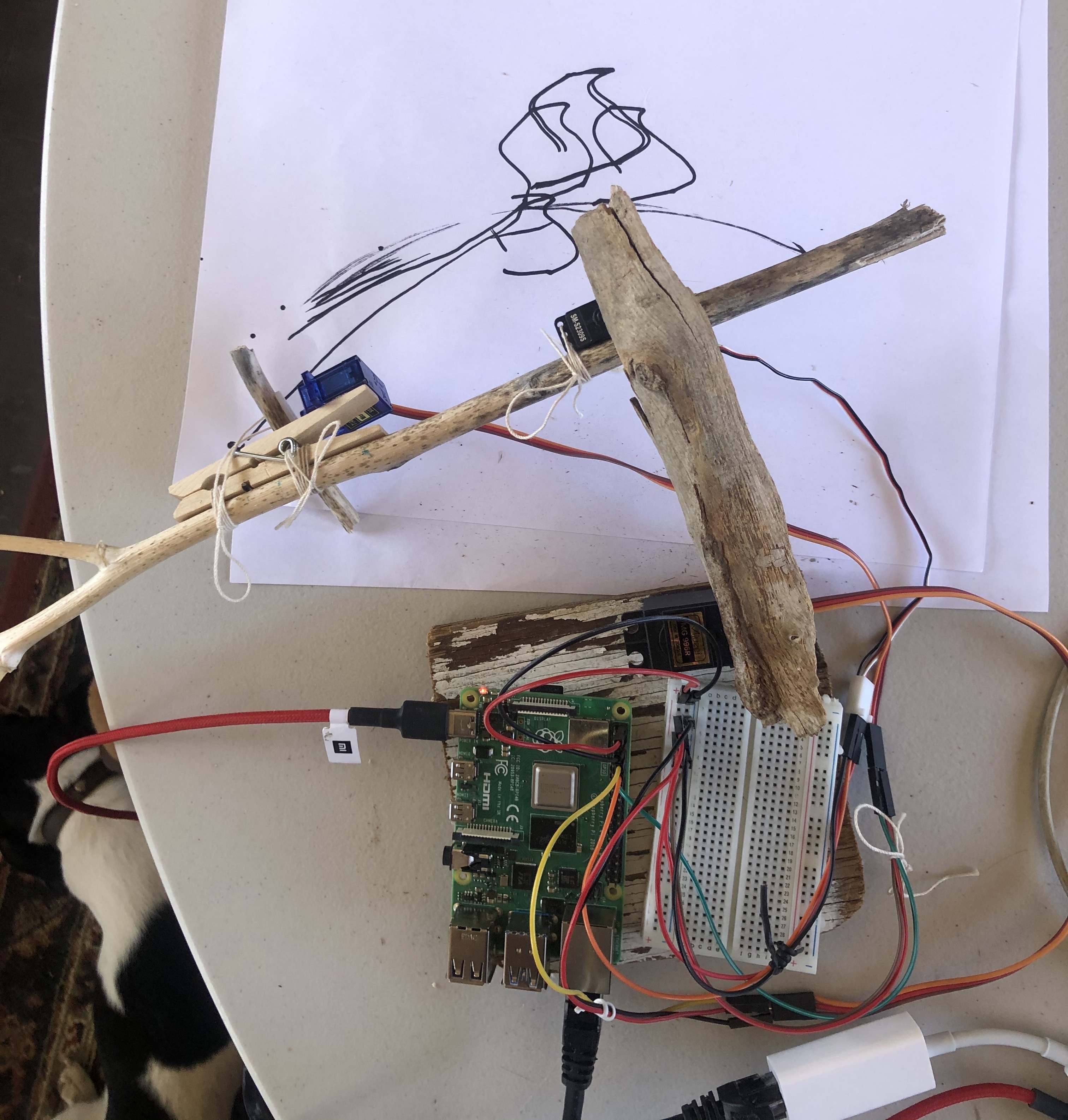
<p>I built a drawing robot with wood found in the desert! The machanism and software is heavily based on <a href="https://brachiograph.readthedocs.io/en/latest/index.html">BranchioGraph</a>, with a different construct and orientation that required some tinkering to figure out.</p>

<p><img src="/assets/img/bbd/15-2.jpeg" alt="robot2" />
<em>very ad-hoc calibration setup ft. printed protractor and earing</em></p>
<p style="width: 60%;" class="center"><img src="/assets/img/bbd/15-3.jpeg" alt="robot3" />
<em>first run! It drew a bonfire.</em></p>

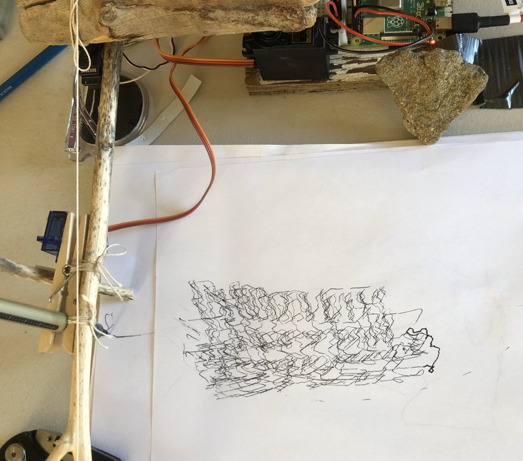
<p>Even after calibration the drawing is still a little… wonky, because of the elasticity in the sticks, the looseness of the joints, and inacuracies of servo controls. In some ways, though, these faults added a layer of intermediacy to the drawing (or the act of drawing), which one may see as part of the machine’s <em>touch</em>.</p>

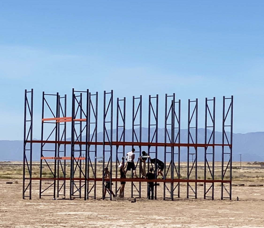
<p style="width: 60%;" class="center"><img src="/assets/img/bbd/13-7.jpeg" alt="pallet racks" />
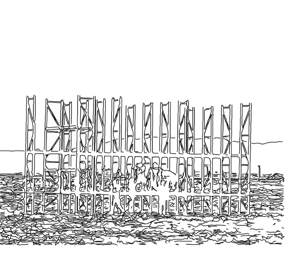
<img src="/assets/img/bbd/15-4.jpeg" alt="vectors" />
<img src="/assets/img/bbd/15-5.jpeg" alt="drawing" />
<em>A drawing of a vectorized picture of us building pallet racks.</em></p>
<p> </p>

<p>The bot even participated in our weekly <em>drink-and-draw</em> event. People blew into a alcohol sensor appended to the raspberry Pi, whose reading were used to parametrize the <code class="language-plaintext highlighter-rouge">open-cv</code> vectorize function. (So technically, we drank and it drew.) Here is <a href="https://twitter.com/_yokaii_/status/1249096320083607553">a video</a> of the bot figure drawing.</p>

<p> 
You may find my code for it <a href="https://github.com/guiguiguiguigui/chatsubo-e">here</a>.</p>]]></content><author><name>Sophia Sun</name></author><category term="projects" /><summary type="html"><![CDATA[]]></summary></entry><entry><title type="html">chicken soup for the cs phd student</title><link href="https://huiwenn.github.io/readings" rel="alternate" type="text/html" title="chicken soup for the cs phd student" /><published>2020-06-02T01:09:00+00:00</published><updated>2020-06-02T01:09:00+00:00</updated><id>https://huiwenn.github.io/readings</id><content type="html" xml:base="https://huiwenn.github.io/readings"><![CDATA[<blockquote>
  <p>Pieces of writings that I found helpful for thinking about research and surviving a PhD.</p>
</blockquote>

<!--more-->

<h3 id="de-mystifying-good-research-and-good-papers-by-fei-fei-li"><em>De-Mystifying Good Research and Good Papers</em>, by Fei-Fei Li</h3>

<p>read it <a href="https://bigaidream.gitbooks.io/tech-blog/content/2014/de-mystifying-good-research.html">here</a>.</p>

<p>I’m putting this one first because it’s a succint yet powerful read. It’s easy to be caught up in the “publish or perish” culture and the race of metric hacking / low-hanging fruits; this article serves as a good reminder of that’s not why we are here doing research.</p>

<blockquote>
  <p>Every research project and every paper should be conducted and written with one singular purpose: to genuinely advance the field of computer vision. So when you conceptualize and carry out your work, you need to be constantly asking yourself this question in the most critical way you could – “Would my work define or reshape xxx (problem, field, technique) in the future?”</p>
</blockquote>

<blockquote>
  <p>This means publishing papers is NOT about “this has not been published or written before, let me do it”, nor is it about “let me find an arcane little problem that can get me an easy poster”. It’s about “if I do this, I could offer a better solution to this important problem,” or “if I do this, I could add a genuinely new and important piece of knowledge to the field.”</p>
</blockquote>

<h3 id="you-and-your-research-by-richard-hamming"><em>You and Your Research</em>, by Richard Hamming</h3>

<p>read it <a href="http://www.cs.virginia.edu/~robins/YouAndYourResearch.html">here</a>.</p>

<p>A classic and important reading for any researcher in science. In his talk (linked is a transcription) Hamming talks about <em>what</em> constitutes <em>important work</em>, <em>why</em> do it, and <em>how</em> to do it. The arguments are interlaced with cool personal science anecdotes and lined with optimism – it reminded me of why I am here doing grad school in the first place. I first heard about the talk’s existence, funnily enough, from <a href="http://www.paulgraham.com/hamming.html">Paul Graham</a>, but I’ve seen scientists I look up to reference it again and agian, from when they’re feeling burnt out to when facing important decisions. It carries a message worth bearing in our minds as we go about, well, being us and doing our research.</p>

<h3 id="the-phd-grind-by-phillip-guo"><em>The PhD Grind</em>, by Phillip Guo</h3>

<p>(update: Phillip took down the book; see his <a href="https://pg.ucsd.edu/index.html#faq">FAQ</a>. you may still find copies online. Perhaps instead, check out his <a href="https://pg.ucsd.edu/early-stage-PhD-advice.htm">Advice for early-stage Ph.D. students</a>.)</p>

<p>The pitch I generally give people about this book is that Phillip encountered a pretty comprehensive set of problems for a CS PhD student, and prevailed (!). In this mini memoir he writes with clarity, provides sound analysis, and offers precious advices. Whatever problem you are experiencing, you are likely to find a way to reason about it from this book. Feel like you are just doing grunt work? Find it hard to communicate with you advisor? Anxious about not publishing (whereby proving your competence)? Deciding between industry vs academia? Phil’s got you.</p>

<p>It is both endearing and inspiring to learn about his journey, and to know that he came out ok (he’s a professor at UCSD now!). I really appreciate the honesty and detail he put into this work. Thank you!</p>

<h2 id="other-interesting-things">Other Interesting things</h2>
<ul>
  <li><a href="http://matt.might.net/articles/phd-school-in-pictures/">An illustrated guide to PhD</a></li>
  <li><a href="https://jiasi.wordpress.com/2019/05/27/invisible-accomplishments/?fbclid=IwAR2nwe6TdMMpt8t2qhDee5WFvPo6vF7trRR8Wwl29ym6DFxTUQTOqsFJl1A">How to transform into a senior PhD student</a></li>
  <li><a href="https://www.amazon.com/PhD-Not-Enough-Survival-Science/dp/0465022227">A PhD Is Not Enough!: A Guide to Survival in Science (book)</a></li>
  <li><a href="http://phdcomics.com/">phd comics</a></li>
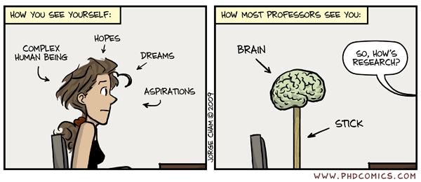
</ul>

<p> </p>

<p><img src="/assets/img/misc/brainstick.gif" alt="brain on a stick" /></p>]]></content><author><name>Sophia Sun</name></author><category term="meta-research" /><summary type="html"><![CDATA[Pieces of writings that I found helpful for thinking about research and surviving a PhD.]]></summary></entry><entry><title type="html">Karaoke of Dreams</title><link href="https://huiwenn.github.io/karaoke" rel="alternate" type="text/html" title="Karaoke of Dreams" /><published>2020-04-01T00:00:00+00:00</published><updated>2020-04-01T00:00:00+00:00</updated><id>https://huiwenn.github.io/karaoke</id><content type="html" xml:base="https://huiwenn.github.io/karaoke"><![CDATA[<!--more-->

<p><img src="/assets/img/karaoke/01-rec.jpg" alt="" />
 
<img src="/assets/img/karaoke/02.jpg" alt="" /></p>

<p> </p>

<p>This is a computer-generated karaoke I built with <a href="https://www.yuditskaya.com/">Sofy</a> and <a href="https://www.derekxkwan.com/">Derek</a> during our time together in <a href="https://brahman.ai/">Brahman.ai</a>, Bombay Beach CA.</p>

<p>For details, please see <a href="/assets/img/idx/KoD.pdf">our paper</a> :)</p>

<p> 
<img src="/assets/img/bbd/9-4.jpg" alt="sofy and the tesseract" />
<em>Sofy building the tesseract.</em></p>]]></content><author><name>Sophia Sun</name></author><category term="projects" /><summary type="html"><![CDATA[]]></summary></entry><entry><title type="html">Trees</title><link href="https://huiwenn.github.io/yuanque" rel="alternate" type="text/html" title="Trees" /><published>2020-03-25T00:00:00+00:00</published><updated>2020-03-25T00:00:00+00:00</updated><id>https://huiwenn.github.io/yuanque</id><content type="html" xml:base="https://huiwenn.github.io/yuanque"><![CDATA[<!--more-->

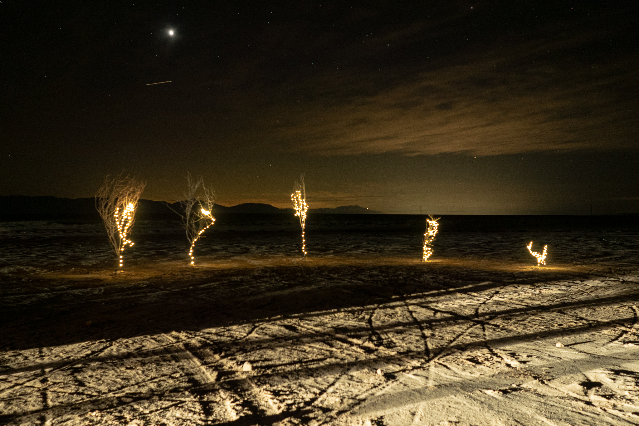
<p><img src="/assets/img/yuanque/t.jpg" alt="" />
 
<img src="/assets/img/yuanque/3.jpg" alt="" />
 </p>

<p>This project is my little attempt at land art. I gathered dead trees from the deseart and replanted them, in a shape that resembles a half moon. Concentric patterns are raked on the ground on some days. Solar-powered LEDs climb the branches, both as a night-time safty measure and as a hint to, in some sense, a new kind of life. I call it 圆缺, Yuan Que, a word for the moon cycle from old chinese poetry.</p>

<p>My friend <a href="https://yinitis.com/">Yin</a> was kind enough to perform an original choreography on this site.</p>

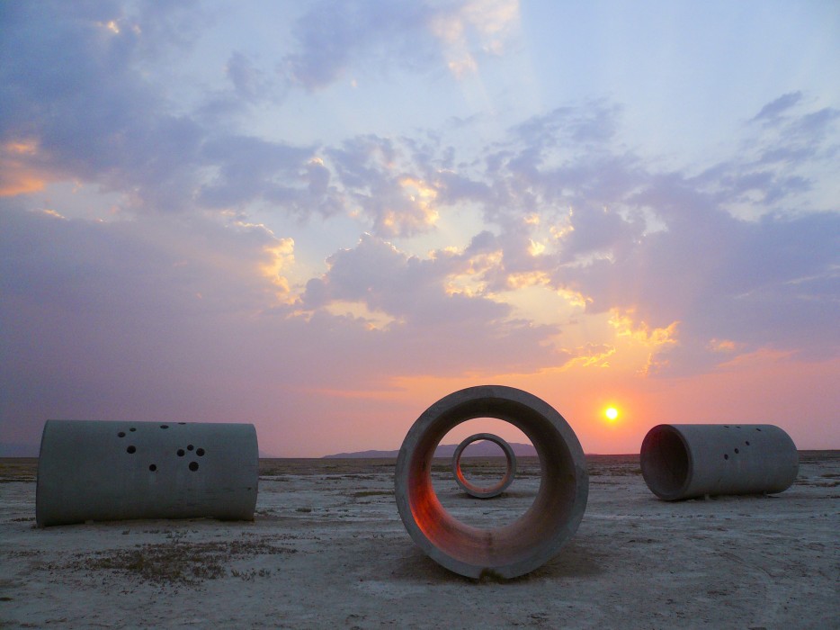
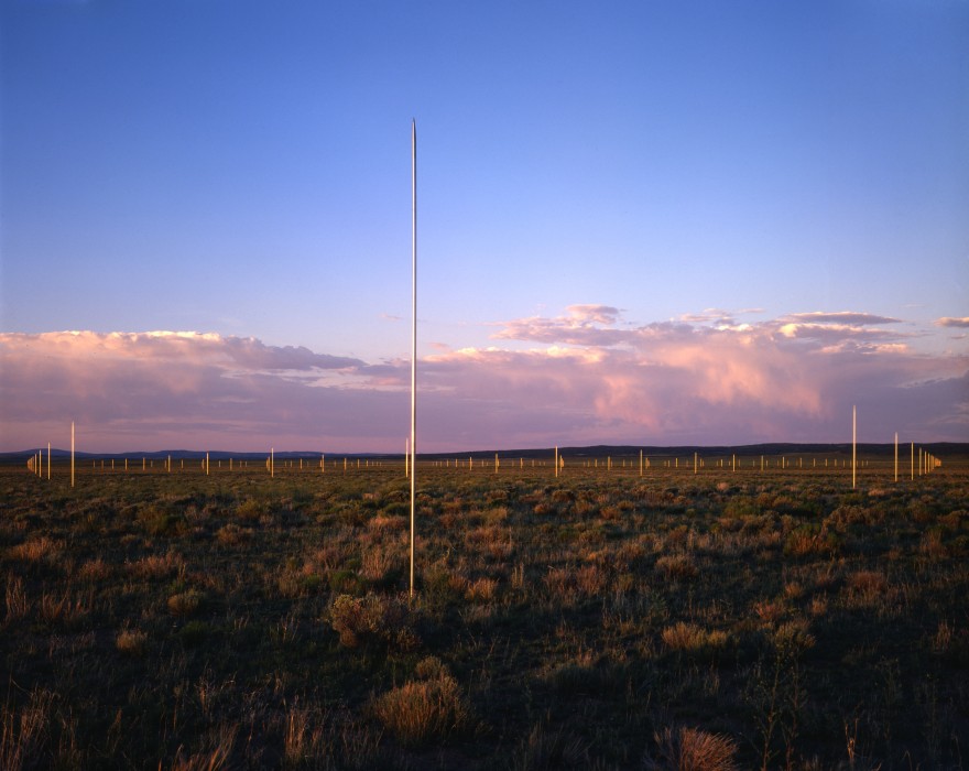
<p>This piece is very much inspired by, and pays homage to, the tradition of land art here in the American west. These pieces have changed how I understand we may live on this overwhelming, open, vast land.</p>

<p> </p>

<p style="width: 80%;" class="center"><img src="/assets/img/yuanque/suntunnels.jpg" alt="Sun Tunnels" />
<em>Nancy Holt, Sun Tunnels, 1973–76. Great Basin Desert, Utah. Photo by James Fox, courtesy Holt/Smithson Foundation</em></p>
<p> </p>

<p style="width: 80%;" class="center"><img src="/assets/img/yuanque/lightning.jpg" alt="Sun Tunnels" />
<em>Walter De Maria, The Lightning Field, 1977. © Estate of Walter De Maria. Photo: John Cliett</em></p>
<p> </p>]]></content><author><name>Sophia Sun</name></author><category term="projects" /><summary type="html"><![CDATA[]]></summary></entry><entry><title type="html">Implementing Self-Tuning Spectral Clustering</title><link href="https://huiwenn.github.io/spectral-clustering" rel="alternate" type="text/html" title="Implementing Self-Tuning Spectral Clustering" /><published>2020-01-10T00:00:00+00:00</published><updated>2020-01-10T00:00:00+00:00</updated><id>https://huiwenn.github.io/spectral-clustering</id><content type="html" xml:base="https://huiwenn.github.io/spectral-clustering"><![CDATA[<blockquote>
  <p>An (attempt at) implementation of the self-tuning spectral clustering algorithm by Zelnik-Manor and Perona (2014).</p>
</blockquote>

<!--more-->

<ul class="table-of-content" id="markdown-toc">
  <li><a href="#spectral-clustering" id="markdown-toc-spectral-clustering">Spectral Clustering</a></li>
  <li><a href="#graph-laplacian" id="markdown-toc-graph-laplacian">Graph Laplacian</a></li>
  <li><a href="#implementing-the-njw-algorithm" id="markdown-toc-implementing-the-njw-algorithm">Implementing the NJW algorithm</a></li>
  <li><a href="#tunning-oneself" id="markdown-toc-tunning-oneself">Tunning Oneself</a>    <ul>
      <li><a href="#local-scaling" id="markdown-toc-local-scaling">Local Scaling</a></li>
      <li><a href="#estimating-number-of-clusters" id="markdown-toc-estimating-number-of-clusters">Estimating number of clusters</a></li>
    </ul>
  </li>
  <li><a href="#image-segmentation" id="markdown-toc-image-segmentation">Image Segmentation</a></li>
  <li><a href="#references" id="markdown-toc-references">References</a></li>
</ul>

<p>This implementation was a homework for a class called <em>Geometry of Data</em> (very cool) taught by <a href="http://mishne.ucsd.edu">Gal Mishne</a> (also very cool).</p>

<p>One thing about CS grad school is that I started encountering problems whose solutions can’t be easily found online or in books (how inconvenient!). Sometimes, though, it makes the process very fulfilling, and this is one of those times.</p>

<h2 id="spectral-clustering">Spectral Clustering</h2>

<p>Spectral clustering is a approach to clustering where we (1) construct a graph from data and then (2) partition the graph by analyzing its connectivity.</p>

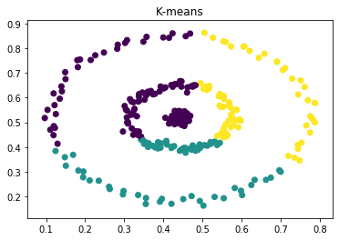
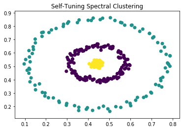
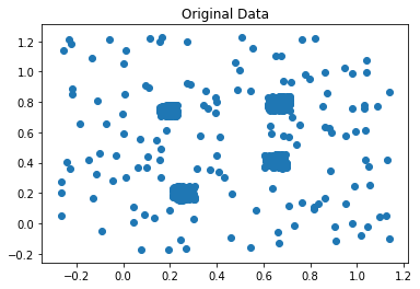
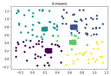
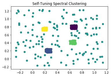
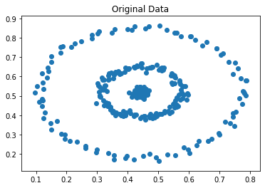
<p>This is a departure from some of the more well-known approaches, such as  K-means or learning a mixture model via EM, which are based on the assumption that clusters are concentrated in terms of (often Cartesian) distance. They tend not to do the best when the clusters are of complex or unknown shape, for example -</p>

<table>
  <tbody>
    <tr>
      <td><img src="/assets/img/clustering/2-og.png" alt="" /></td>
      <td><img src="/assets/img/clustering/2-kmeans.png" alt="" /></td>
      <td><img src="/assets/img/clustering/2-sc.png" alt="" /></td>
    </tr>
  </tbody>
</table>

<p><em><center>figure 1: concentric circles</center></em></p>

<p>hubs and backgrounds:</p>

<table>
  <tbody>
    <tr>
      <td><img src="/assets/img/clustering/1-og.png" alt="" /></td>
      <td><img src="/assets/img/clustering/1-kmeans.png" alt="" /></td>
      <td><img src="/assets/img/clustering/1-sc2.png" alt="" /></td>
    </tr>
  </tbody>
</table>

<p><em><center>figure 2: two different densities</center></em></p>

<h2 id="graph-laplacian">Graph Laplacian</h2>

<p>The clustering algorithm is made possible by a very handy property of the graph Laplacian.</p>

<p>The Laplacian matrix of a graph \(G\) with \(n\) nodes is defined as</p>

\[L = D - A\]

<p>where \(D\) is the degree matrix and \(A\) is the adjacency matrix of graph \(G\). In other words, \(L\) is an \(n \times n\) matrix with elements given by</p>

\[L_{i,j} = \begin{cases}
                        \text{deg}(v_i) &amp; \text{if } i=j \\
                        -w_{i,j} &amp; \text{if } i \neq j \text{ and there is an edge between i and j }\\
                        0 &amp; \text{otherwise }
                    \end{cases}\]

<p>If \(G\) is unweighted, we can use \(w_{i,j} = 1\) for each edge.</p>

<p>The property we will be taking advantage of is:</p>
<blockquote>
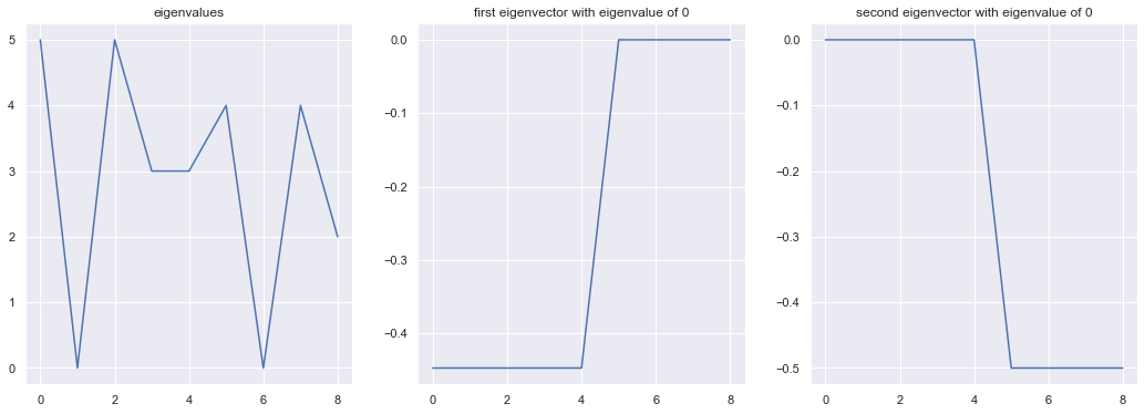
  <p>If the graph \(G\) has \(K\) connected components, then \(L\) has \(K\) eigenvectors with an eigenvalue of 0.</p>
</blockquote>

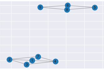
<p>Moreover, the eigenvectors with eigenvalue of 0 are organized in terms of value to indicate the connected components. Here’s an example, with code from <a href="https://towardsdatascience.com/unsupervised-machine-learning-spectral-clustering-algorithm-implemented-from-scratch-in-python-205c87271045">Cory Maklin’s blog post</a>:</p>

<div class="language-python highlighter-rouge"><div class="highlight"><pre class="highlight"><code><span class="kn">import</span> <span class="nn">networkx</span> <span class="k">as</span> <span class="n">nx</span>
<span class="kn">import</span> <span class="nn">numpy</span> <span class="k">as</span> <span class="n">np</span>

<span class="n">G</span> <span class="o">=</span> <span class="n">nx</span><span class="p">.</span><span class="n">Graph</span><span class="p">()</span>
<span class="n">G</span><span class="p">.</span><span class="n">add_edges_from</span><span class="p">([[</span><span class="mi">1</span><span class="p">,</span> <span class="mi">2</span><span class="p">],</span> <span class="p">[</span><span class="mi">1</span><span class="p">,</span> <span class="mi">3</span><span class="p">],</span> <span class="p">[</span><span class="mi">1</span><span class="p">,</span> <span class="mi">4</span><span class="p">],</span>  <span class="p">[</span><span class="mi">2</span><span class="p">,</span> <span class="mi">3</span><span class="p">],</span>
                 <span class="p">[</span><span class="mi">2</span><span class="p">,</span> <span class="mi">7</span><span class="p">],</span> <span class="p">[</span><span class="mi">3</span><span class="p">,</span> <span class="mi">4</span><span class="p">],</span> <span class="p">[</span><span class="mi">4</span><span class="p">,</span> <span class="mi">7</span><span class="p">],</span> <span class="p">[</span><span class="mi">1</span><span class="p">,</span> <span class="mi">7</span><span class="p">],</span>
                 <span class="p">[</span><span class="mi">6</span><span class="p">,</span> <span class="mi">5</span><span class="p">],</span> <span class="p">[</span><span class="mi">5</span><span class="p">,</span> <span class="mi">8</span><span class="p">],</span> <span class="p">[</span><span class="mi">6</span><span class="p">,</span> <span class="mi">8</span><span class="p">],</span>  <span class="p">[</span><span class="mi">9</span><span class="p">,</span> <span class="mi">8</span><span class="p">],</span> <span class="p">[</span><span class="mi">9</span><span class="p">,</span> <span class="mi">6</span><span class="p">]])</span>
<span class="n">draw_graph</span><span class="p">(</span><span class="n">G</span><span class="p">)</span>
<span class="n">A</span> <span class="o">=</span> <span class="n">nx</span><span class="p">.</span><span class="n">adjacency_matrix</span><span class="p">(</span><span class="n">G</span><span class="p">)</span>
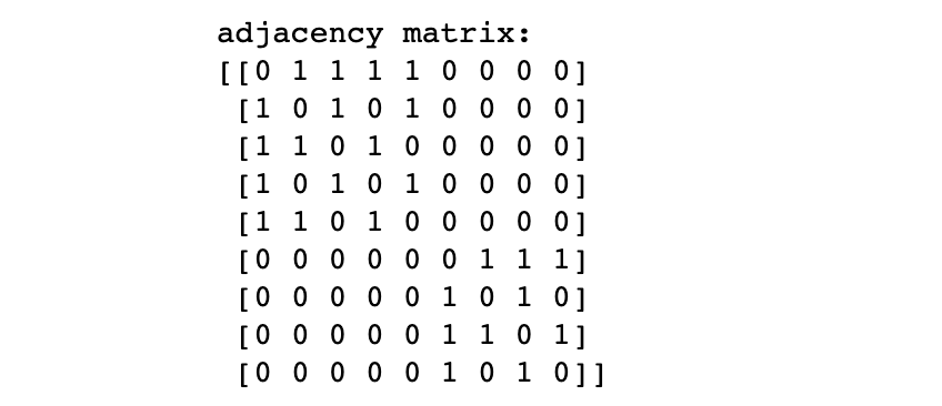
<span class="k">print</span><span class="p">(</span><span class="s">'adjacency matrix:'</span><span class="p">)</span>
<span class="k">print</span><span class="p">(</span><span class="n">A</span><span class="p">.</span><span class="n">todense</span><span class="p">())</span>
</code></pre></div></div>

<table>
  <tbody>
    <tr>
      <td><img src="/assets/img/clustering/laplacian-1.png" alt="" /></td>
      <td><img src="/assets/img/clustering/lap-a.png" alt="" /></td>
    </tr>
  </tbody>
</table>

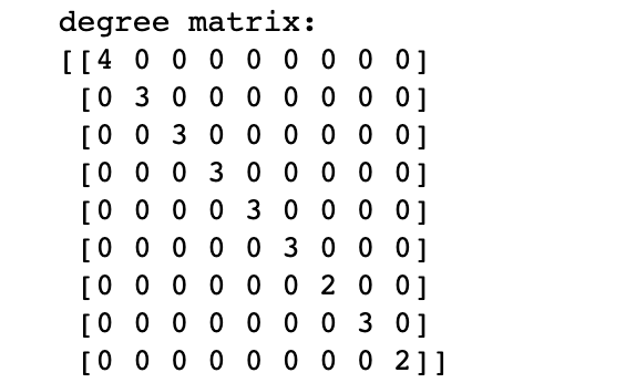
<div class="language-python highlighter-rouge"><div class="highlight"><pre class="highlight"><code><span class="n">D</span> <span class="o">=</span> <span class="n">np</span><span class="p">.</span><span class="n">diag</span><span class="p">(</span><span class="n">np</span><span class="p">.</span><span class="nb">sum</span><span class="p">(</span><span class="n">np</span><span class="p">.</span><span class="n">array</span><span class="p">(</span><span class="n">A</span><span class="p">.</span><span class="n">todense</span><span class="p">()),</span> <span class="n">axis</span><span class="o">=</span><span class="mi">1</span><span class="p">))</span>
<span class="k">print</span><span class="p">(</span><span class="s">'degree matrix:'</span><span class="p">)</span>
<span class="k">print</span><span class="p">(</span><span class="n">D</span><span class="p">)</span>

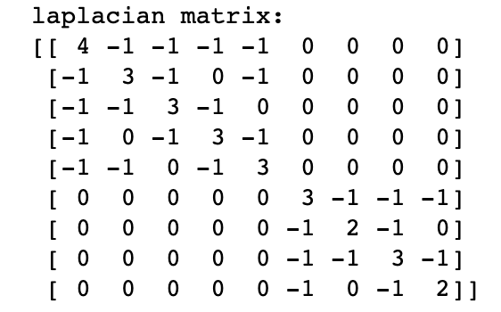
<span class="n">L</span> <span class="o">=</span> <span class="n">D</span> <span class="o">-</span> <span class="n">A</span>
<span class="k">print</span><span class="p">(</span><span class="s">'laplacian matrix:'</span><span class="p">)</span>
<span class="k">print</span><span class="p">(</span><span class="n">L</span><span class="p">)</span>
</code></pre></div></div>

<table>
  <tbody>
    <tr>
      <td><img src="/assets/img/clustering/lap-d.png" alt="" /></td>
      <td><img src="/assets/img/clustering/lap-l.png" alt="" /></td>
    </tr>
  </tbody>
</table>

<p> </p>

<p>Now, if we calculate the eigenvalues and eigenvectors of the Laplacian, we get two 0 eigenvalues as expected. The eigenvectors corresponding to them clearly separate the two clusters. In practice, we use k-means to separate the clusters across the eigenvectors (see section below), as even the clusters are not cleanly separated, the eigenvectors still provide information about interconnectivity.</p>

<p> </p>

<p><img src="/assets/img/clustering/eigen.png" alt="" />
<em>figure 3: concentric circles</em></p>

<p> </p>

<p>TODO: but what does a graph Laplacian and its eigenvectors <em>mean</em>?</p>

<h2 id="implementing-the-njw-algorithm">Implementing the NJW algorithm</h2>

<p>Here we follow Ng, Jordan, and Weiss’s algorithm <a href="#references">[2]</a> for (not self-tuning) spectral clustering and implement it step by step. It goes like this:</p>

<p>Given a set of points \(S= \{s_1, \ldots, s_n\}\) in \(\mathbb{R}^l\) and desired number of clusters \(k\):</p>

<ol>
  <li>
    <p>Calculate affinity matrix \(A \in \mathbb{R}^{n \times n}\) defined by</p>

\[A_{ij} = \begin{cases} \exp (- \| s_i - s_j \| ^2 / 2 \sigma^2) &amp; \text{for } i \neq j\\  0 &amp; \text{for } i=j \end{cases}\]

    <div class="language-python highlighter-rouge"><div class="highlight"><pre class="highlight"><code> <span class="kn">import</span> <span class="nn">numpy</span> <span class="k">as</span> <span class="n">np</span>
 <span class="kn">from</span> <span class="nn">scipy.spatial.distance</span> <span class="kn">import</span> <span class="n">pdist</span> <span class="c1">#Calculates pairwise distance
</span>
 <span class="k">def</span> <span class="nf">make_A</span><span class="p">(</span><span class="n">X</span><span class="p">,</span> <span class="n">sigma</span><span class="p">):</span>
     <span class="n">dim</span> <span class="o">=</span> <span class="n">X</span><span class="p">.</span><span class="n">shape</span><span class="p">[</span><span class="mi">0</span><span class="p">]</span>
     <span class="n">A</span> <span class="o">=</span> <span class="n">np</span><span class="p">.</span><span class="n">zeros</span><span class="p">([</span><span class="n">dim</span><span class="p">,</span> <span class="n">dim</span><span class="p">])</span>
     <span class="n">dist</span> <span class="o">=</span> <span class="nb">iter</span><span class="p">(</span><span class="n">pdist</span><span class="p">(</span><span class="n">X</span><span class="p">))</span>
     <span class="k">for</span> <span class="n">i</span> <span class="ow">in</span> <span class="nb">range</span><span class="p">(</span><span class="n">dim</span><span class="p">):</span>
         <span class="k">for</span> <span class="n">j</span> <span class="ow">in</span> <span class="nb">range</span><span class="p">(</span><span class="n">i</span><span class="o">+</span><span class="mi">1</span><span class="p">,</span> <span class="n">dim</span><span class="p">):</span>  
             <span class="n">d</span> <span class="o">=</span> <span class="n">np</span><span class="p">.</span><span class="n">exp</span><span class="p">(</span><span class="o">-</span><span class="mi">1</span><span class="o">*</span><span class="nb">next</span><span class="p">(</span><span class="n">dist</span><span class="p">)</span><span class="o">**</span><span class="mi">2</span><span class="o">/</span><span class="p">(</span><span class="n">sigma</span><span class="o">**</span><span class="mi">2</span><span class="p">))</span>
             <span class="n">A</span><span class="p">[</span><span class="n">i</span><span class="p">,</span><span class="n">j</span><span class="p">]</span> <span class="o">=</span> <span class="n">d</span>
             <span class="n">A</span><span class="p">[</span><span class="n">j</span><span class="p">,</span><span class="n">i</span><span class="p">]</span> <span class="o">=</span> <span class="n">d</span>
     <span class="k">return</span> <span class="n">A</span>
</code></pre></div>    </div>
  </li>
  <li>
    <p>Define \(D\) to be the diagonal matrix whose \((i,i)\) element is the sum of \(A\)’s \(i\)-th row, and construct the Laplacian \(L = D^{-1/2}A D^{-1/2}\).</p>

    <div class="language-python highlighter-rouge"><div class="highlight"><pre class="highlight"><code> <span class="kn">from</span> <span class="nn">scipy</span> <span class="kn">import</span> <span class="n">linalg</span>

 <span class="n">A</span> <span class="o">=</span> <span class="n">make_A</span><span class="p">(</span><span class="n">data</span><span class="p">,</span> <span class="mf">0.3</span><span class="p">)</span> <span class="c1">#Hyper parameter for sigma
</span> <span class="n">D</span> <span class="o">=</span> <span class="n">np</span><span class="p">.</span><span class="nb">sum</span><span class="p">(</span><span class="n">A</span><span class="p">,</span> <span class="n">axis</span><span class="o">=</span><span class="mi">0</span><span class="p">)</span> <span class="o">*</span> <span class="n">np</span><span class="p">.</span><span class="n">eye</span><span class="p">(</span><span class="n">X</span><span class="p">.</span><span class="n">shape</span><span class="p">[</span><span class="mi">0</span><span class="p">])</span>
 <span class="n">D_half</span> <span class="o">=</span> <span class="n">linalg</span><span class="p">.</span><span class="n">fractional_matrix_power</span><span class="p">(</span><span class="n">D</span><span class="p">,</span> <span class="o">-</span><span class="mf">0.5</span><span class="p">)</span>
 <span class="n">L</span> <span class="o">=</span> <span class="n">np</span><span class="p">.</span><span class="n">matmul</span><span class="p">(</span><span class="n">np</span><span class="p">.</span><span class="n">matmul</span><span class="p">(</span><span class="n">D_half</span><span class="p">,</span> <span class="n">A</span><span class="p">),</span> <span class="n">D_half</span><span class="p">)</span>
</code></pre></div>    </div>
  </li>
  <li>
    <p>Find the \(k\) largest distinct eigenvectors \(x_1, x_2 , \ldots, x_k\) and form the matrix \(X = [x_1x_2\dots x_k]\) by stacking them together as columns.</p>

    <div class="language-python highlighter-rouge"><div class="highlight"><pre class="highlight"><code> <span class="c1"># numpy returns the eigenvectors as a matrix where the 
</span> <span class="c1"># i-th column corresponds to the i-th eigenvalue.
</span> <span class="c1"># In the case of all real eigenvalues, they are organized from
</span> <span class="c1"># small to large. So we are taking the slice of the last k columns.
</span> <span class="n">eigval</span><span class="p">,</span> <span class="n">eigvec</span> <span class="o">=</span> <span class="n">np</span><span class="p">.</span><span class="n">linalg</span><span class="p">.</span><span class="n">eigh</span><span class="p">(</span><span class="n">L</span><span class="p">)</span> 
 <span class="n">X</span> <span class="o">=</span> <span class="n">eigvec</span><span class="p">[:,</span> <span class="o">-</span><span class="mi">1</span><span class="o">*</span><span class="n">k</span><span class="p">:]</span>
</code></pre></div>    </div>
  </li>
  <li>Re-normalize each row of \(X\) to have unit length. Denote \(Y_{ij} = X_{ij}/(\sum_j X_{ij}^2)^{1/2}\). This step is algorithmically cosmetic and deals with difference of connectivity within a cluster; one may skip this step if that gives better results empirically.
    <div class="language-python highlighter-rouge"><div class="highlight"><pre class="highlight"><code> <span class="n">row_sums</span> <span class="o">=</span> <span class="n">Y</span><span class="p">.</span><span class="nb">sum</span><span class="p">(</span><span class="n">axis</span><span class="o">=</span><span class="mi">1</span><span class="p">)</span>
 <span class="n">Y</span> <span class="o">=</span> <span class="n">Y</span> <span class="o">/</span> <span class="n">row_sums</span><span class="p">[:,</span> <span class="n">np</span><span class="p">.</span><span class="n">newaxis</span><span class="p">]</span>
</code></pre></div>    </div>
  </li>
  <li>Cluster each row of \(Y\) into \(k\) clusters by K-means or any other algorithm.
    <div class="language-python highlighter-rouge"><div class="highlight"><pre class="highlight"><code> <span class="kn">from</span> <span class="nn">sklearn.cluster</span> <span class="kn">import</span> <span class="n">KMeans</span>
 <span class="n">clusters</span> <span class="o">=</span> <span class="n">KMeans</span><span class="p">(</span><span class="n">n_clusters</span><span class="o">=</span><span class="n">k</span><span class="p">).</span><span class="n">fit</span><span class="p">(</span><span class="n">Y</span><span class="p">).</span><span class="n">labels_</span>
</code></pre></div>    </div>
  </li>
  <li>Assign the original point \(s_i\) to the cluster \(j\) where the \(i\)-th row of matrix \(Y\) was assigned to. Implementation-wise, we reuse the <code class="language-plaintext highlighter-rouge">clusters</code> variable directly.</li>
</ol>

<p>To finish up, here’s two lines for plotting -</p>

<div class="language-python highlighter-rouge"><div class="highlight"><pre class="highlight"><code><span class="kn">import</span> <span class="nn">matplotlib.pyplot</span> <span class="k">as</span> <span class="n">plt</span>

<span class="n">plt</span><span class="p">.</span><span class="n">scatter</span><span class="p">(</span><span class="n">X</span><span class="p">[:,</span><span class="mi">0</span><span class="p">],</span> <span class="n">X</span><span class="p">[:,</span><span class="mi">1</span><span class="p">],</span> <span class="n">c</span> <span class="o">=</span> <span class="n">clusters</span><span class="p">)</span>
<span class="n">plt</span><span class="p">.</span><span class="n">title</span><span class="p">(</span><span class="s">"Spectral Clustering"</span><span class="p">)</span>
</code></pre></div></div>

<h2 id="tunning-oneself">Tunning Oneself</h2>

<h3 id="local-scaling">Local Scaling</h3>
<p>The main drawback of the global \(\sigma\) hyperparameter is that it does not handle the case where data is of various density across the domain, for which a \(\sigma\) may work well with some portion of the data but not the rest. (see figure TODO for example.)</p>

<p>Zelnik-Manor and Perona [1] argues that connectivity/affinity (matrix \(A\)) should be viewed from the points themselves. We can formulate it by selecting a local scaling parameter for each data point \(s_i\).
The distance from \(s_i\) to \(s_j\) from the perspective of \(s_i\) is \(d(s_i , s_j )/\sigma_i\) and the converse is  \(d(s_i , s_j )/\sigma_j\). The square distance may be generalized as their product, i.e. \(d(s_i , s_j )^2/\sigma_i \sigma_j\). The (local-scaled) affinity between a pair of points therefore becomes:</p>

\[\hat{A}_{ij} = \exp(\frac{-d(s_i,s_j)^2}{\sigma_i\sigma_j})\]

<p>Having such construct allows us to adapt the distance -&gt; affinity scaling to data’s local landscape. One way of achieving this goal, as introduced in [1], is to use the local nearest neighbor statistics</p>

\[\sigma_i = d(s_i, s_K)\]

<p>Where \(s_K\) is the \(K\)‘th neighbor of \(s_i\). So instead of a graph whose edge weight is absolute distance, we want to construct a weighted nearest neighbor graph. Hyperparameter \(K\) will need to be manually tuned ([1] states that \(K=7\) worked well for all their experiments).</p>

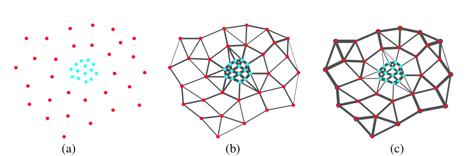
<p>Take data in the following figure for example. The local-scaled affinity will be high between points that are <em>both</em> close neighbors to each other, whereby strongly connecting the red points as in (c) rather than in (b) where a single global \(\sigma\) is used.</p>

<p style="width: 80%;" class="center"><img src="/assets/img/clustering/local-scaling.png" alt="figure 2" />
<em>Effect of local scaling, figure 2 from [1]. (a) input data point (b) affinity unscaled, and (c) affinity after local scaling</em></p>
<p>The implementation of self tuning is straightforward.</p>

<div class="language-python highlighter-rouge"><div class="highlight"><pre class="highlight"><code><span class="kn">from</span> <span class="nn">tqdm</span> <span class="kn">import</span> <span class="n">tqdm</span>

<span class="k">def</span> <span class="nf">A_local</span><span class="p">(</span><span class="n">X</span><span class="p">):</span>
    <span class="n">dim</span> <span class="o">=</span> <span class="n">X</span><span class="p">.</span><span class="n">shape</span><span class="p">[</span><span class="mi">0</span><span class="p">]</span>
    <span class="n">dist_</span> <span class="o">=</span> <span class="n">pdist</span><span class="p">(</span><span class="n">X</span><span class="p">)</span>
    <span class="n">pd</span> <span class="o">=</span> <span class="n">np</span><span class="p">.</span><span class="n">zeros</span><span class="p">([</span><span class="n">dim</span><span class="p">,</span> <span class="n">dim</span><span class="p">])</span>
    <span class="n">dist</span> <span class="o">=</span> <span class="nb">iter</span><span class="p">(</span><span class="n">dist_</span><span class="p">)</span>
    <span class="k">for</span> <span class="n">i</span> <span class="ow">in</span> <span class="nb">range</span><span class="p">(</span><span class="n">dim</span><span class="p">):</span>
        <span class="k">for</span> <span class="n">j</span> <span class="ow">in</span> <span class="nb">range</span><span class="p">(</span><span class="n">i</span><span class="o">+</span><span class="mi">1</span><span class="p">,</span> <span class="n">dim</span><span class="p">):</span>  
            <span class="n">d</span> <span class="o">=</span> <span class="nb">next</span><span class="p">(</span><span class="n">dist</span><span class="p">)</span>
            <span class="n">pd</span><span class="p">[</span><span class="n">i</span><span class="p">,</span><span class="n">j</span><span class="p">]</span> <span class="o">=</span> <span class="n">d</span>
            <span class="n">pd</span><span class="p">[</span><span class="n">j</span><span class="p">,</span><span class="n">i</span><span class="p">]</span> <span class="o">=</span> <span class="n">d</span>
            
    <span class="c1">#calculate local sigma
</span>    <span class="n">sigmas</span> <span class="o">=</span> <span class="n">np</span><span class="p">.</span><span class="n">zeros</span><span class="p">(</span><span class="n">dim</span><span class="p">)</span>
    <span class="k">for</span> <span class="n">i</span> <span class="ow">in</span> <span class="n">tqdm</span><span class="p">(</span><span class="nb">range</span><span class="p">(</span><span class="nb">len</span><span class="p">(</span><span class="n">pd</span><span class="p">))):</span>
        <span class="n">sigmas</span><span class="p">[</span><span class="n">i</span><span class="p">]</span> <span class="o">=</span> <span class="nb">sorted</span><span class="p">(</span><span class="n">pd</span><span class="p">[</span><span class="n">i</span><span class="p">])[</span><span class="mi">7</span><span class="p">]</span>
    
    <span class="n">A</span> <span class="o">=</span> <span class="n">np</span><span class="p">.</span><span class="n">zeros</span><span class="p">([</span><span class="n">dim</span><span class="p">,</span> <span class="n">dim</span><span class="p">])</span>
    <span class="n">dist</span> <span class="o">=</span> <span class="nb">iter</span><span class="p">(</span><span class="n">dist_</span><span class="p">)</span>
    <span class="k">for</span> <span class="n">i</span> <span class="ow">in</span> <span class="n">tqdm</span><span class="p">(</span><span class="nb">range</span><span class="p">(</span><span class="n">dim</span><span class="p">)):</span>
        <span class="k">for</span> <span class="n">j</span> <span class="ow">in</span> <span class="nb">range</span><span class="p">(</span><span class="n">i</span><span class="o">+</span><span class="mi">1</span><span class="p">,</span> <span class="n">dim</span><span class="p">):</span>  
            <span class="n">d</span> <span class="o">=</span> <span class="n">np</span><span class="p">.</span><span class="n">exp</span><span class="p">(</span><span class="o">-</span><span class="mi">1</span><span class="o">*</span><span class="nb">next</span><span class="p">(</span><span class="n">dist</span><span class="p">)</span><span class="o">**</span><span class="mi">2</span><span class="o">/</span><span class="p">(</span><span class="n">sigmas</span><span class="p">[</span><span class="n">i</span><span class="p">]</span><span class="o">*</span><span class="n">sigmas</span><span class="p">[</span><span class="n">j</span><span class="p">]))</span>
            <span class="c1">#print(d)
</span>            <span class="n">A</span><span class="p">[</span><span class="n">i</span><span class="p">,</span><span class="n">j</span><span class="p">]</span> <span class="o">=</span> <span class="n">d</span>
            <span class="n">A</span><span class="p">[</span><span class="n">j</span><span class="p">,</span><span class="n">i</span><span class="p">]</span> <span class="o">=</span> <span class="n">d</span>
    <span class="k">return</span> <span class="n">A</span>
</code></pre></div></div>

<p>We can then plug the affinity matrix <em>A</em> into step 2-6 of the NJW algorithm and get results shown in figure 1 and 2.</p>

<h3 id="estimating-number-of-clusters">Estimating number of clusters</h3>

<p>So far, all the algorithms we discussed requires the number of cluster as a hyper parameter. In practical cases, however, the optimal number of clusters is often unclear.</p>

<p>Zelnik-Manor and Perona (2014)’s algorithm proposes to use non-maximal suppression after rotating the eigenvector to estimate the number of groups.</p>

<h2 id="image-segmentation">Image Segmentation</h2>

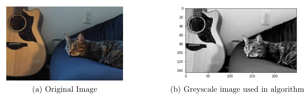
<p>One use case of clustering is on image segmentation. I happen to be cat-sitting for my friend as I’m writing this assignment, so here we go.</p>

<p><img src="/assets/img/clustering/cat.png" alt="cat" />
<em>🎸🛋️🐈</em></p>

<p>The way I approached it is to cut the image into smaller patches and cluster them. The code below resizes the image matrix into non-overlapping patches of size \(2×2\), essentially down-sampling the image. <code class="language-plaintext highlighter-rouge">open-cv</code>’s python package is used for this processing.</p>

<div class="language-python highlighter-rouge"><div class="highlight"><pre class="highlight"><code><span class="kn">import</span> <span class="nn">cv2</span>
<span class="kn">from</span> <span class="nn">sklearn.feature_extraction</span> <span class="kn">import</span> <span class="n">image</span>

<span class="n">im_</span> <span class="o">=</span> <span class="n">cv2</span><span class="p">.</span><span class="n">imread</span><span class="p">(</span><span class="s">"img_small.jpg"</span><span class="p">,</span> <span class="n">cv2</span><span class="p">.</span><span class="n">IMREAD_COLOR</span><span class="p">)</span>
<span class="n">im</span> <span class="o">=</span> <span class="n">cv2</span><span class="p">.</span><span class="n">cvtColor</span><span class="p">(</span><span class="n">im_</span><span class="p">,</span> <span class="n">cv2</span><span class="p">.</span><span class="n">COLOR_BGR2GRAY</span><span class="p">)</span>
<span class="n">plt</span><span class="p">.</span><span class="n">imshow</span><span class="p">(</span><span class="n">im</span><span class="p">,</span> <span class="n">cmap</span> <span class="o">=</span> <span class="s">'gray'</span><span class="p">)</span> 

<span class="n">sz</span> <span class="o">=</span> <span class="n">im</span><span class="p">.</span><span class="n">itemsize</span>
<span class="n">h</span><span class="p">,</span><span class="n">w</span> <span class="o">=</span> <span class="n">im</span><span class="p">.</span><span class="n">shape</span>
<span class="n">bh</span><span class="p">,</span><span class="n">bw</span> <span class="o">=</span> <span class="mi">2</span><span class="p">,</span><span class="mi">2</span> <span class="c1">#block height and width
</span><span class="n">shape</span> <span class="o">=</span> <span class="p">(</span><span class="nb">int</span><span class="p">(</span><span class="n">h</span><span class="o">/</span><span class="n">bh</span><span class="p">),</span> <span class="nb">int</span><span class="p">(</span><span class="n">w</span><span class="o">/</span><span class="n">bw</span><span class="p">),</span> <span class="n">bh</span><span class="p">,</span> <span class="n">bw</span><span class="p">)</span>
<span class="n">strides</span> <span class="o">=</span> <span class="n">sz</span><span class="o">*</span><span class="n">np</span><span class="p">.</span><span class="n">array</span><span class="p">([</span><span class="n">w</span><span class="o">*</span><span class="n">bh</span><span class="p">,</span><span class="n">bw</span><span class="p">,</span><span class="n">w</span><span class="p">,</span><span class="mi">1</span><span class="p">])</span>
<span class="k">print</span><span class="p">(</span><span class="n">shape</span><span class="p">,</span> <span class="n">strides</span><span class="p">)</span>

<span class="n">patches</span> <span class="o">=</span> <span class="n">np</span><span class="p">.</span><span class="n">lib</span><span class="p">.</span><span class="n">stride_tricks</span><span class="p">.</span><span class="n">as_strided</span><span class="p">(</span><span class="n">im</span><span class="p">,</span> <span class="n">shape</span><span class="o">=</span><span class="n">shape</span><span class="p">,</span> <span class="n">strides</span><span class="o">=</span><span class="n">strides</span><span class="p">)</span>
</code></pre></div></div>

<p>Then we apply the algorithm we implemented on the patches. This step is computationally intense and thus time consuming, so I recommend saving the matrices as they are being computed.</p>

<div class="language-python highlighter-rouge"><div class="highlight"><pre class="highlight"><code><span class="n">a</span><span class="p">,</span><span class="n">b</span><span class="p">,</span><span class="n">c</span><span class="p">,</span><span class="n">d</span> <span class="o">=</span> <span class="n">patches</span><span class="p">.</span><span class="n">shape</span>
<span class="n">X</span> <span class="o">=</span> <span class="n">patches</span><span class="p">.</span><span class="n">reshape</span><span class="p">([</span><span class="n">a</span><span class="o">*</span><span class="n">b</span><span class="p">,</span> <span class="n">c</span><span class="o">*</span><span class="n">d</span><span class="p">])</span>
<span class="n">A</span> <span class="o">=</span> <span class="n">A_local</span><span class="p">(</span><span class="n">X</span><span class="p">)</span>
<span class="n">D_half</span> <span class="o">=</span> <span class="n">linalg</span><span class="p">.</span><span class="n">fractional_matrix_power</span><span class="p">(</span><span class="n">np</span><span class="p">.</span><span class="nb">sum</span><span class="p">(</span><span class="n">A</span><span class="p">,</span> <span class="n">axis</span><span class="o">=</span><span class="mi">0</span><span class="p">)</span> <span class="o">*</span> <span class="n">np</span><span class="p">.</span><span class="n">eye</span><span class="p">(</span><span class="n">X</span><span class="p">.</span><span class="n">shape</span><span class="p">[</span><span class="mi">0</span><span class="p">]),</span> <span class="o">-</span><span class="mf">0.5</span><span class="p">)</span>
<span class="n">L</span> <span class="o">=</span> <span class="n">np</span><span class="p">.</span><span class="n">matmul</span><span class="p">(</span><span class="n">np</span><span class="p">.</span><span class="n">matmul</span><span class="p">(</span><span class="n">D_half</span><span class="p">,</span> <span class="n">A</span><span class="p">),</span> <span class="n">D_half</span><span class="p">)</span>

<span class="n">eigval</span><span class="p">,</span> <span class="n">eigvec</span> <span class="o">=</span> <span class="n">np</span><span class="p">.</span><span class="n">linalg</span><span class="p">.</span><span class="n">eigh</span><span class="p">(</span><span class="n">L</span><span class="p">)</span>
</code></pre></div></div>

<p>we can then plot the eigenvectors.</p>

<div class="language-python highlighter-rouge"><div class="highlight"><pre class="highlight"><code><span class="k">def</span> <span class="nf">eig2pic_</span><span class="p">(</span><span class="n">eig</span><span class="p">):</span>
    <span class="n">arr_blocks</span> <span class="o">=</span> <span class="n">eig</span><span class="p">.</span><span class="n">reshape</span><span class="p">([</span><span class="n">a</span><span class="p">,</span> <span class="n">b</span><span class="p">])</span> <span class="c1">#a, b comes from code block above
</span>    <span class="n">img</span> <span class="o">=</span> <span class="n">np</span><span class="p">.</span><span class="n">array</span><span class="p">([</span><span class="n">np</span><span class="p">.</span><span class="n">hstack</span><span class="p">(</span><span class="n">bl</span><span class="p">)</span> <span class="k">for</span> <span class="n">bl</span> <span class="ow">in</span> <span class="n">arr_blocks</span><span class="p">])</span>
    <span class="n">img</span> <span class="o">=</span> <span class="n">np</span><span class="p">.</span><span class="n">vstack</span><span class="p">(</span><span class="n">img</span><span class="p">)</span>
    <span class="n">plt</span><span class="p">.</span><span class="n">imshow</span><span class="p">(</span><span class="n">img</span><span class="p">,</span> <span class="n">cmap</span> <span class="o">=</span> <span class="s">'gray'</span><span class="p">)</span> 

<span class="n">eig2pic_</span><span class="p">(</span><span class="n">eigvec_cat</span><span class="p">[:,</span><span class="o">-</span><span class="mi">1</span><span class="p">])</span>
</code></pre></div></div>

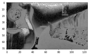
<p><img src="/assets/img/clustering/e-1.png" alt="eig-1" />
<em>Largest Eigenvector.</em></p>

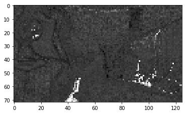
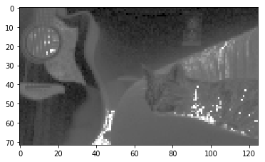
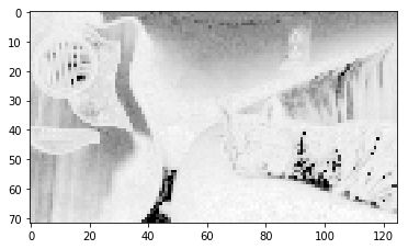
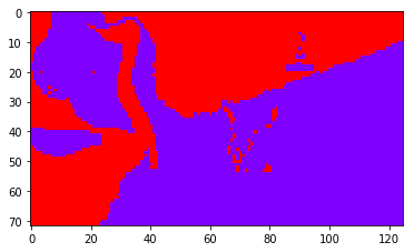
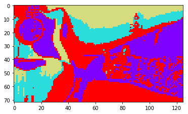
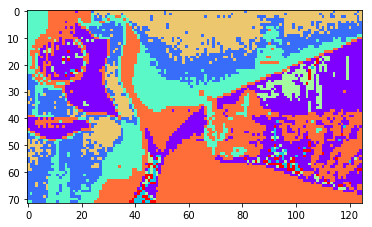
<p>Note that the boundaries of the guitar and part of the cat are marked with darker lines, signifying segmentation boundaries. The next few eigenvectors indicates other modes of segmentation:</p>

<table>
  <tbody>
    <tr>
      <td><img src="/assets/img/clustering/e-2.png" alt="" /></td>
      <td><img src="/assets/img/clustering/e-3.png" alt="" /></td>
      <td><img src="/assets/img/clustering/e-4.png" alt="" /></td>
    </tr>
  </tbody>
</table>

<p> </p>

<p>And here are some segmentation results with k-means ran on the first \(k\) eigenvectors, with \(k=2\), \(k=4\), \(k=8\).</p>

<table>
  <tbody>
    <tr>
      <td><img src="/assets/img/clustering/c-2.png" alt="" /></td>
      <td><img src="/assets/img/clustering/c-4.png" alt="" /></td>
      <td><img src="/assets/img/clustering/c-8.png" alt="" /></td>
    </tr>
  </tbody>
</table>

<p> </p>

<p>Thanks for reading!
<img src="/assets/img/clustering/cat.jpeg" alt="" /></p>

<h2 id="references">References</h2>

<p>[1] Lihi Zelnik-Manor, Pietro Perona. <a href="https://arxiv.org/abs/1902.01342">“Self-Tuning Spectral Clustering”</a> NeurIPS 2014.</p>

<p>[2] Andrew Ng, Michael Jordan and Yair Weiss. <a href="https://www.semanticscholar.org/paper/On-Spectral-Clustering%3A-Analysis-and-an-algorithm-Ng-Jordan/c02dfd94b11933093c797c362e2f8f6a3b9b8012">“On spectral clustering: Analysis and an algorithm”</a> NeurIPS 2001.</p>

<p>[3] Carl Doersch, Abhinav Gupta, and Alexei A. Efros. <a href="https://arxiv.org/abs/1505.05192">“Unsupervised visual representation learning by context prediction.”</a> ICCV. 2015.</p>]]></content><author><name>Sophia Sun</name></author><category term="machine-learning" /><summary type="html"><![CDATA[An (attempt at) implementation of the self-tuning spectral clustering algorithm by Zelnik-Manor and Perona (2014).]]></summary></entry></feed>